Next: Density of States Per
Up: Lecture 2
Previous: Seebeck Effect - Thermopower
(``Free
Electrons; Sommerfeld")
(AM, Ch 2)
Now let's put  into the model.
The most important effect of putting quantum mechanics into the
theory of metals is the result of treating electrons as fermions with
Fermi-Dirac statistics, rather than as a classical gas of particles
obeying the Kinetic Theory of Gases. But let's start at the
beginning.
When electrons are treated quantum mechanically, 2 things change: (a)
possible states are quantized; (b) particles are indistinguishable.
=2.0 true in
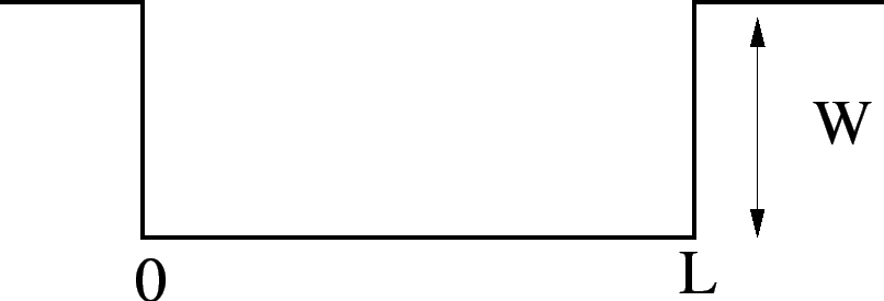
What boundary conditions do we use? (It doesn't matter all that much
because the bulk properties aren't really affected by what goes on at
the surface.)
- (a)
- Realistic, i.e.,
 finite outside the metal but
decaying exponentially
finite outside the metal but
decaying exponentially  as
as
 ). This is
practically never used for bulk calculations since
). This is
practically never used for bulk calculations since
 atomic dimensions.
- (b)
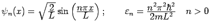
- Box: Standing Wave Solutions
 at walls
 .
.
We're interested in transport - want traveling waves.
- (c)
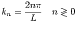
- Periodic:
Now traveling wave solutions are allowed.
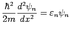
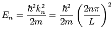
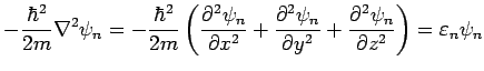
It is easy to generalize this to 3D. Consider a box with sides
 : Schroedinger's equation becomes
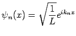
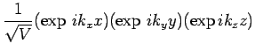
For periodic b.c.'s, the solution is a product wavefunction
with
The momentum carried in the plane wave state is
 and the velocity
 . Each state is characterized by
  and by the spin
  along some chosen axis. There are 2 different states for each
allowed value of . Note that the probability density
along some chosen axis. There are 2 different states for each
allowed value of . Note that the probability density
 is uniform in space.
Density of States
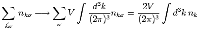
Suppose we are interested in some property of the
one-electron states, such as the total average number of electrons in
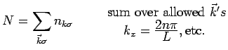
them. We sum over the states
where
 is the number of electrons in state
  with
spin .
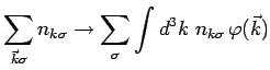
Assume that
is a rather smoothly varying function of
. This allows us to transform the sum into an integral.
with
spin .
Assume that
is a rather smoothly varying function of
. This allows us to transform the sum into an integral.
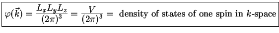
 is the density of states per unit volume of
-space. What is
?
is the density of states per unit volume of
-space. What is
?
 implies that the density of allowed
  values along the
-axis is
values along the
-axis is
 . Similar
arguments for
. Similar
arguments for  and
and  lead to
Note that this is independent of the ratio of
lead to
Note that this is independent of the ratio of  , and
, and  .
In fact,
is independent of the sample shape in the
limit
.
In fact,
is independent of the sample shape in the
limit
 , except for the lowest few states.
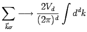
If spin is included, put in an extra factor of 2. Thus
if
is independent of . In general for any
dimension 
where  is the -dimensional volume.
Next: Density of States Per
Up: Lecture 2
Previous: Seebeck Effect - Thermopower
Clare Yu
2006-10-03