Next: About this document ...
Physics 115A: Statistical Physics
Prof. Clare Yu
email: cyu@uci.edu
phone: 949-824-6216
Office: 210E RH
Spring 2009
LECTURE 1
Introduction
So far your physics courses have concentrated on what happens to
one object or a few objects given an external potential and perhaps
the interactions between objects. For example, Newton's second law  refers to the mass of the object and its acceleration.
In quantum mechanics, one starts with Schroedinger's equation
refers to the mass of the object and its acceleration.
In quantum mechanics, one starts with Schroedinger's equation  and
solves it to find the wavefunction
and
solves it to find the wavefunction  which describes a particle.
But if you look around you, the world has more than a few particles and
objects. The air you breathe and the coffee you drink has lots and lots
of atoms and molecules. Now you might think that if we can describe each
atom or molecule with what we know from classical mechanics, quantum
mechanics, and electromagnetism, we can just scale up and describe
10
which describes a particle.
But if you look around you, the world has more than a few particles and
objects. The air you breathe and the coffee you drink has lots and lots
of atoms and molecules. Now you might think that if we can describe each
atom or molecule with what we know from classical mechanics, quantum
mechanics, and electromagnetism, we can just scale up and describe
10 particles. That's like saying that if you can cook dinner for
3 people, then just scale up the recipe and feed the world. The reason
we can't just take our solution for the single particle problem and
multiply by the number of particles in a liquid or a gas is that the particles
interact with one another, i.e., they apply a force on each other. They
see the potential produced by other particles. This makes things really
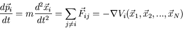
complicated. Suppose we have a system of N interacting particles.
Using Newton's equations, we would write:
particles. That's like saying that if you can cook dinner for
3 people, then just scale up the recipe and feed the world. The reason
we can't just take our solution for the single particle problem and
multiply by the number of particles in a liquid or a gas is that the particles
interact with one another, i.e., they apply a force on each other. They
see the potential produced by other particles. This makes things really
complicated. Suppose we have a system of N interacting particles.
Using Newton's equations, we would write:
 |
(1) |
where  is the force on the
  th particle produced by
the
th particle produced by
the  th particle.
  is the total potential energy of the th
particle assuming that all the forces are conservative. We must also
specify the initial conditions, i.e., the initial positions and velocities
of all the particles. Then we must solve the N coupled second order partial
differential equations. This is quite a daunting task. It's true that
we now have powerful computers and molecular dynamics simulations carry
out such tasks, but they can only handle a few thousand particles and
track their motions for perhaps a 10
is the total potential energy of the th
particle assuming that all the forces are conservative. We must also
specify the initial conditions, i.e., the initial positions and velocities
of all the particles. Then we must solve the N coupled second order partial
differential equations. This is quite a daunting task. It's true that
we now have powerful computers and molecular dynamics simulations carry
out such tasks, but they can only handle a few thousand particles and
track their motions for perhaps a 10 seconds. So we throw up
our hands. This is not the way to go.
seconds. So we throw up
our hands. This is not the way to go.
Fortunately, there is a better way. We can use the fact that there are
large numbers of particles to apply a statistical analysis to the situation.
We are usually not interested in the detailed microscopics of a liquid or
a gas. Instead we are usually interested in certain macroscopic quantities like
- pressure
- temperature
- entropy
- specific heat
- electrical conductivity
- magnetic and electric susceptibilities
- etc.
These concepts don't make sense for one atom or even a few particles.
For example, what is the temperature of one atom? That doesn't make sense.
But if we have a whole bucket of atoms, then temperature makes sense.
Since we are not concerned with the detailed behavior of each and every
particle, we can use statistical methods to extract information about
a system with  interacting particles. For example, we may be interested
in the average energy of the system, rather than the energy of each particle.
Statistical methods work best when there are large numbers of particles.
(Think of polling.) Typically we have on the order of a mole's worth
of particles. A mole is the number of atoms contained in 12 grams of
carbon 12. (A carbon 12 atom has 6 protons and 6 neutrons for a total
12 nucleons. Its atomic weight is 12.) So a mole has
interacting particles. For example, we may be interested
in the average energy of the system, rather than the energy of each particle.
Statistical methods work best when there are large numbers of particles.
(Think of polling.) Typically we have on the order of a mole's worth
of particles. A mole is the number of atoms contained in 12 grams of
carbon 12. (A carbon 12 atom has 6 protons and 6 neutrons for a total
12 nucleons. Its atomic weight is 12.) So a mole has
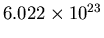 atoms. This is called Avogadro's number.
There are two basic approaches to describing the properties of a large
number of particles:
- Thermodynamics: This is essentially a postulational approach,
or a deductive approach. On the basis of a few general assumptions, general
relationships between and among macroscopic parameters are deduced. No
reference is made to the microscopic details of the system.
- Statistical Mechanics: This is an inductive approach. With only
a few assumptions, relations between the macroscopic parameters of a system
are induced from a consideration of the microscopic interactions. This
approach yields all of the thermodynamic results plus a good deal more
information about the system of interacting particles.
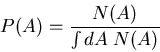
Probability
We will talk more about probability in the discussion section.
If we flip a coin, the chance of heads is 1/2 and the chance of tails is 1/2.
The probability of an outcome is the number of ways of getting that outcome
divided by the total number of outcomes. We often write  for the
probability that an outcome is
for the
probability that an outcome is  . So if we flip 2 coins, then
P(head,head)=1/4, and P(head,tail)=1/2 because there are a total of
4 possible outcomes and 2 ways of getting one coin heads and one
coin tails.
. So if we flip 2 coins, then
P(head,head)=1/4, and P(head,tail)=1/2 because there are a total of
4 possible outcomes and 2 ways of getting one coin heads and one
coin tails.
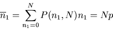
Binary Model
Let's work out a simple example of a binary model. Rather
than heads or tails, think of a line of spins which can be up ( )
or down (
)
or down ( ). The spins correspond to magnetic moments
  .
.
 corresponds to and
  corresponds to .
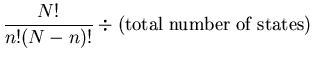
Suppose we have N sites, each with a spin. On each site the spin can
be up or down. The total number of arrangements is
corresponds to .
Suppose we have N sites, each with a spin. On each site the spin can
be up or down. The total number of arrangements is
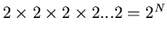 . So the total number of states
or outcomes is
. So the total number of states
or outcomes is  . We can denote a state by
 |
(2) |
Now suppose we want the number of configurations with n up sites,
regardless of what order they're in. The number of down sites will
be N-n, since the total number of sites is N. The number of such
configurations is
 |
(3) |
To see where this comes from, suppose we have N spins of which n are up
and (N-n) are down. How many ways are there to arrange them?
Recall that the number of ways to arrange N objects with one object
on each site (or in each box) is
- the first place can be occupied by any one of the N objects
- the second place can be occupied by any one of the N-1 remaining objects
etc. until the last place can be occupied by the last 1 object.
So there are
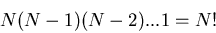 |
(4) |
configurations. In these configurations the
n up spins can be arranged in any of  ways. Also the remaining
(N-n) sites have down spins which can be arranged in any of
ways. Also the remaining
(N-n) sites have down spins which can be arranged in any of  ways.
The spins are regarded as distinguishable. So there are 2 ways to have
ways.
The spins are regarded as distinguishable. So there are 2 ways to have
 :
and
. They
look the same, but if one were red and the other blue, you would see the
difference (red, blue) and (blue, red). We are dividing out this
overcounting; that's what the denominator
:
and
. They
look the same, but if one were red and the other blue, you would see the
difference (red, blue) and (blue, red). We are dividing out this
overcounting; that's what the denominator  is for.
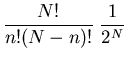
So the probability of a state with n up spins and (N-n) down spins
is
Now suppose that the probability of a site getting is  and the
probability of getting is
and the
probability of getting is  . So far we have considered
up and down to be equally probable, so
. So far we have considered
up and down to be equally probable, so  . But what if
 ? This might be caused by
an external magnetic field which biases the spins one way or another.
If we have 2 spins, the probability of getting 2 up spins is
? This might be caused by
an external magnetic field which biases the spins one way or another.
If we have 2 spins, the probability of getting 2 up spins is  . (Recall
that the probability of flipping a coin twice and getting heads both
times is 1/4.) If we want n up spins and (N-n) down spins, then the
probability is
. (Recall
that the probability of flipping a coin twice and getting heads both
times is 1/4.) If we want n up spins and (N-n) down spins, then the
probability is
When , this reduces to our previous result (5).
Equation (6) is called the binomial distribution because
the prefactor  is the coefficient in the binomial expansion:
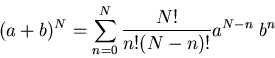 |
(7) |
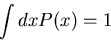
Normalization, Averages, Second Moment
Let's go back to our general considerations of probability
distribution functions.
Let be the probability distribution for the probability that
an outcome is . If we sum over all possible outcomes, one of them
is bound to happen, so
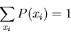 |
(8) |
In other words, the probability distribution function is normalized to
one. One can also have a probability distribution function
 of a continuous variable
  . For example, suppose you leave a meter
stick outside on the ground.
. For example, suppose you leave a meter
stick outside on the ground.  could be the probability that the
first raindrop to hit the stick will strike between position and
could be the probability that the
first raindrop to hit the stick will strike between position and  .
is called the probability density.
The normalization condition is
.
is called the probability density.
The normalization condition is
 |
(9) |
Note that  is the area under the curve . The normalization
sets this area equal to 1.
is the area under the curve . The normalization
sets this area equal to 1.
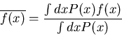
The average of some quantity is
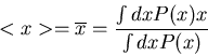 |
(10) |
Averages can be denoted by  or
or  . For a discrete quantity
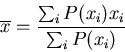 |
(11) |
If the probability is normalized, then the denominator is 1. For example,
suppose  is the number of people with age
  . Then the
average age is
. Then the
average age is
The probability that a person is  old is
 |
(13) |
Notice that this satisfies the normalization condition. More generally,
if  is a function of , then the average value of is
 |
(14) |
One of the more useful functions concerns the deviation of
from the mean :
 |
(15) |
Then
A more useful quantity is the square of the deviation from the mean
This is known as the second moment of about its mean. The first moment
is just .
In general the nth moment of about its mean is given by
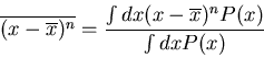 |
(18) |
Two other terms that are often used are the most probable value of x and
the median. The most probable value of is the maximum of . The median
 is the value of such that half the values of are greater
than , i.e.,
is the value of such that half the values of are greater
than , i.e.,  , and half the values of are less
than , i.e.,
, and half the values of are less
than , i.e.,  . In terms of the area under the curve,
the median is the vertical dividing line such that half the area lies to the left
of the median and half to the right of the median.
. In terms of the area under the curve,
the median is the vertical dividing line such that half the area lies to the left
of the median and half to the right of the median.
Gaussian Distribution and Central Limit Theorem
One of most useful distributions is the Gaussian distribution. This is
sometimes called the bell curve which is well known as the ideal grade
distribution.
=3.5 true in
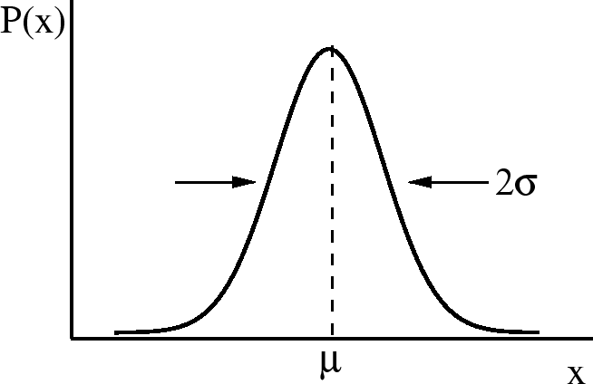
The formula for a Gaussian distribution is
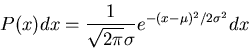 |
(19) |
where
 is the mean.
The coefficient is set so that the normalization condition is satisfied.
is the mean.
The coefficient is set so that the normalization condition is satisfied.
 .
.
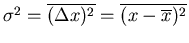
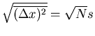
 is the width of the distribution. There is a 68% chance that
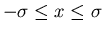 . One obtains this by integrating from
 to
to  .
.  is sometimes called the
root-mean-square (rms) deviation or the standard deviation.
You will have the opportunity to check some of
these assertions in your homework.
is sometimes called the
root-mean-square (rms) deviation or the standard deviation.
You will have the opportunity to check some of
these assertions in your homework.
For a Gaussian distribution, all the higher moments can be expressed in
terms of the first and second moments. For example
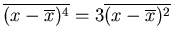 .
.
There is one other interesting aspect of Gaussian distributions. It's called
the central limit theorem. It can be stated in terms of a
random walk in one dimension. A drunk
starts at a lamp post and staggers back and forth along the one
dimensional sidewalk. Let  be the probability that a step length
lies in the range between
be the probability that a step length
lies in the range between  and
and  . No matter what the probability
distribution
. No matter what the probability
distribution  for each step may be, as long as the steps are
statistically independent and falls off rapidly enough as
for each step may be, as long as the steps are
statistically independent and falls off rapidly enough as
 , the total displacement will be distributed
according to the Gaussian law if the number of steps
, the total displacement will be distributed
according to the Gaussian law if the number of steps  is sufficiently
large. This is called the central limit theorem. It is probably the most
famous theorem in mathematical probability theory. The generality of the
result also accounts for the fact that so many phenomena in nature
(e.g., errors in measurement) obey approximately a Gaussian distribution.
is sufficiently
large. This is called the central limit theorem. It is probably the most
famous theorem in mathematical probability theory. The generality of the
result also accounts for the fact that so many phenomena in nature
(e.g., errors in measurement) obey approximately a Gaussian distribution.
In fact, if we go back to the binomial distribution
given in eq. (6), then in the limit of large N, this becomes
the Gaussian distribution (see Reif 1.5). In this case,
represents the net magnetization,
i.e., the difference between the number of up and down spins:
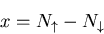 |
(20) |
The average magnetization
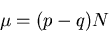 |
(21) |
and the mean square deviation is
 |
(22) |
More on the Random Walk
(Reference: Howard C. Berg, Random Walks in Biology.)
The random walk is an important concept. Let us go back to the drunk starting
at the lamp post and stumbling either to the right or the left. Consider an
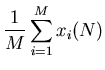
ensemble of M drunks. Let  be the position of the th drunk after
steps. Suppose everyone starts at the origin so that
be the position of the th drunk after
steps. Suppose everyone starts at the origin so that
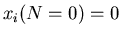 for all . Let the step size be of fixed length . Then
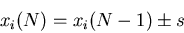 |
(23) |
The average displacement from the origin is
So the mean displacement is zero because on average, half of the displacements
are negative and half are positive. But this does not mean that all the drunks are
sitting at the origin after steps.
It is useful to look at the spread in positions. A convenient measure of spreading
is the root-mean-square (rms) displacement  . Here we average
the square of the displacement rather than the displacement itself. Since the
square of a negative or a positive number is positive, the result will be positive.
. Here we average
the square of the displacement rather than the displacement itself. Since the
square of a negative or a positive number is positive, the result will be positive.
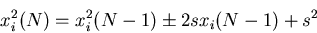 |
(25) |
Then we compute the mean,
So
 ,
,
 ,
,
 ,...,
and
,...,
and
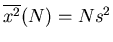 . So the rms displacement
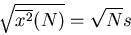 |
(27) |
The rms displacement is a good measure of the typical distance that the drunk reaches.
Notice that it goes as the square root of the number of steps. If  is the
time between successive steps, then it takes a time
is the
time between successive steps, then it takes a time  to take
steps. So
to take
steps. So
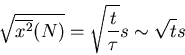 |
(28) |
Notice that the rms displacement goes as square root of the time  .
.
A random walk is what particles execute when the diffuse. Think of a opening
a bottle of perfume. The perfume molecules diffuse through the air. We can
define a diffusion coefficient  by
by
 |
(29) |
(The factor of 2 is by convention.) Then in one dimension
For 2 dimensions, if the x and y directions are independent,
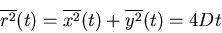 |
(31) |
Similarly for 3 dimensions
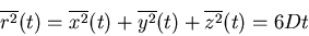 |
(32) |
Notice that in all dimensions, the mean square displacement is linear in
the number of steps and in the time .
The diffusion coefficient characterizes the migration of particles in a given
kind of medium at a given temperature. In general, it depends on the size of the
particle, the structure of the medium, and the absolute temperature. For a small
molecule in water at room temperature,
 cm
cm /sec.
/sec.
If we go back to the drunk who is taking steps of size to the right or to the
left, then we can use the binomial distribution. Let be the probability to
take a step to the right and be the probability to take a step to the
left. After taking steps, the mean number
 of steps to the
right is (see Reif Eq. (1.4.4)):
of steps to the
right is (see Reif Eq. (1.4.4)):
 |
(33) |
The mean number of steps to the left is
 |
(34) |
Let the displacement be
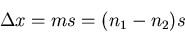 |
(35) |
The mean displacement is (Reif Eq. (1.4.6)):
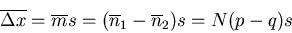 |
(36) |
So if , then the mean displacement
 .
.
The displacement squared is
 |
(37) |
The dispersion of the net displacement or the mean square displacement is
 |
(38) |
where we used Reif Eq. (1.4.12). If , then the mean square displacement
 which is what we got before. The rms displacement is
 |
(39) |
If , then the rms displacement is
 which is what we got before.
Notice again that the rms displacement goes as the square root of the number
of steps. Again the characteristic or typical displacement is given by
which is what we got before.
Notice again that the rms displacement goes as the square root of the number
of steps. Again the characteristic or typical displacement is given by
 .
.
Poisson Distribution
(Ref.: C. Kittel, Thermal Physics)
It is worth mentioning another widely used distribution, namely, the Poisson
distribution. This distribution is concerned with the occurrence of small
numbers of objects in random sampling processes. For example, if on average
there is one bad penny in 1000, what is the probability that no bad
pennies will be found in a given sample of 100 pennies? The problem was
first consided and solved by Poisson (1837) in a study of the role of
luck in criminal and civil trials in France. So suppose that there are
trials and the probability for a desired outcome is . The probability
that there will be  desired outcomes is
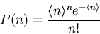 |
(40) |
where the mean number of desired events is
 . You
will derive the Poisson distribution in your homework starting from the
binomial distribution.
. You
will derive the Poisson distribution in your homework starting from the
binomial distribution.
Quantum Mechanics
Since you are just starting your quantum mechanics course, let's just go
over what you need to know for starters. Mostly it's just notation and jargon.
Particles or systems of particles are described by a wavefunction .
The wavefunction is a function of the coordinates of the particles
or of their momenta, but not both. You can't specify both the
momentum and position of a particle because of the Heisenberg
uncertainty principle
 |
(41) |
So the wavefunction of a particle is written  .
The wavefunction is determined by Schroedinger's equation
.
The wavefunction is determined by Schroedinger's equation
 |
(42) |
where  is the Hamiltonian and
  is the energy. The Hamiltonian
is the sum of the kinetic and potential energies. You solve
Schroedinger's equation to determine the wavefunction. Schroedinger's
equation can be written as a matrix equation or as a second order differential
equation. Often the
wavefunction solutions are labeled by definite values of energy,
momentum, etc. These values can only have discrete values, i.e.,
they are quantized. They are called quantum numbers. We can label
the different wavefunction solutions by their quantum numbers.
Quantum numbers correspond to conserved quantities like energy,
momentum, angular momentum, spin angular momentum, etc.
Perhaps the most familiar example of this is the electronic orbitals
in the hydrogen atom. The electron orbitals, like the 1s and 2p states,
have definite discrete energies and definite values of the orbital angular
momentum. For example, the energy of the 1s state in hydrogen is 1 Rydberg
or 13.6 eV. The electron in this state can be described by a wavefunction
is the energy. The Hamiltonian
is the sum of the kinetic and potential energies. You solve
Schroedinger's equation to determine the wavefunction. Schroedinger's
equation can be written as a matrix equation or as a second order differential
equation. Often the
wavefunction solutions are labeled by definite values of energy,
momentum, etc. These values can only have discrete values, i.e.,
they are quantized. They are called quantum numbers. We can label
the different wavefunction solutions by their quantum numbers.
Quantum numbers correspond to conserved quantities like energy,
momentum, angular momentum, spin angular momentum, etc.
Perhaps the most familiar example of this is the electronic orbitals
in the hydrogen atom. The electron orbitals, like the 1s and 2p states,
have definite discrete energies and definite values of the orbital angular
momentum. For example, the energy of the 1s state in hydrogen is 1 Rydberg
or 13.6 eV. The electron in this state can be described by a wavefunction
 . The quantum numbers of this state are
  and
and  .
means that it has energy
.
means that it has energy  eV and
  is the orbital angular
momentum. ( is the spectroscopic notation for .) Solving the
Schroedinger equation for the hydrogen atom yields many wavefunctions
or orbitals (1s, 2s, 2p
is the orbital angular
momentum. ( is the spectroscopic notation for .) Solving the
Schroedinger equation for the hydrogen atom yields many wavefunctions
or orbitals (1s, 2s, 2p , 2p
, 2p , 2p
, 2p , 3s, etc.).
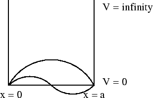
Another example is a particle in a box.
The energy eigenvalues
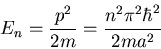 |
(43) |
Each value of corresponds to a different eigenvalue of the energy  .
Notice that the energy levels are not equally spaced; they get farther
apart as you go up in energy.
Each value of also corresponds to a different wavefunction
.
Notice that the energy levels are not equally spaced; they get farther
apart as you go up in energy.
Each value of also corresponds to a different wavefunction
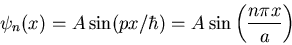 |
(44) |
Notice that the more nodes there are, the more wiggles there are, and
the higher the energy is.
A harmonic oscillator is another example. This is just the
quantum mechanical case of a mass attached to a spring.
In this case the potential
is a parabola rather than being a square well. A particle of mass  in this potential oscillates with frequency
  .
The Hamiltonian is
.
The Hamiltonian is
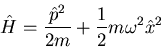 |
(45) |
You will learn how to solve this in your quantum mechanics course. Let me
just write down the result. The energy eigenvalues are
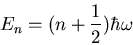 |
(46) |
where 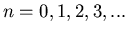 . Notice once again that the energy levels are
quantized. In this case they are evenly spaced by an amount
. Notice once again that the energy levels are
quantized. In this case they are evenly spaced by an amount
 .
The harmonic oscillator has Gaussian wavefunctions
(Hermite polynomials).
.
The harmonic oscillator has Gaussian wavefunctions
(Hermite polynomials).
Wavefunctions can describe more than one particle. You can have a
wavefunction associated with a state with many particles. We call this a
many body wavefunction.
In this case we can describe a state with particles by
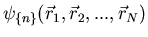 . The subscript
 denotes the quantum numbers that label the wavefunction.
Next: About this document ...
Clare Yu
2009-05-06
![$\displaystyle \frac{1}{M}\sum_{i=1}^{M}\left[x_i(N)=x_i(N-1)\pm s\right]$](img101.png)
![$\displaystyle \frac{1}{M}\sum_{i=1}^{M}\left[x^2_i(N-1)\pm 2sx_i(N-1)+s^2\right]$](img108.png)