Next: About this document ...
Previous: lecture1
Motivation for course
The title of this course is
``condensed matter physics" which
includes solids and liquids (and occasionally gases). There are
also intermediate forms of matter, e.g., glasses, rubber, polymers,
and some biophysical systems. Basically this is the branch of
physics that covers the things we see and touch in everyday
life, i.e., ``real stuff.'' Most of the materials we meet in every
day life are amorphous, but since we understand crystalline materials
so much better, that is what we will spend most of our time talking
about.
Why should we study condensed matter physics?
- ``Because it's there."
- Real-life physics
- Frontier of complexity - ``more is different"
Think of a spin - a multitude gives all sorts of magnetism due to interactions
- Analogies with elementary particle physics, e.g., Higgs
mechanism, topological winding numbers, broken symmetry, etc.
- Practical applications, e.g., transistors.
Drude Theory of Metals
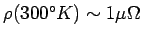
(a) Phenomenology of metals - high electrical conductivity,
shiny (reflecting), ductile + malleable, high thermal conductivity,
etc. Found generally in columns 1A and 2A of the periodic table, among
heavier III-VI column elements, and in transition metals and rare
earths. In general, they have 1-2 extra electrons above a closed
shell. Typically
 few
few
 -cm versus
 -cm for insulators like
polystyrene.
-cm for insulators like
polystyrene.
(b) Basic concepts - The extra electrons are called conduction
electrons and they are free to move within the volume. Core electrons
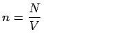
stay home. The number of conduction electrons
where  is the chemical valence
(see table 1.1 of AM). Electronic density is often defined in terms
of
is the chemical valence
(see table 1.1 of AM). Electronic density is often defined in terms
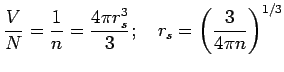
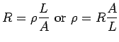
of  radius of sphere whose volume is equal to the volume per
conduction electron:
radius of sphere whose volume is equal to the volume per
conduction electron:
Typically
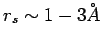 . Natural unit is Bohr radius
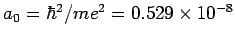 cm.
cm.
For comparison, note that a typical atomic (ionic) radius is
 . So conduction electrons occupy a larger sphere than ions.
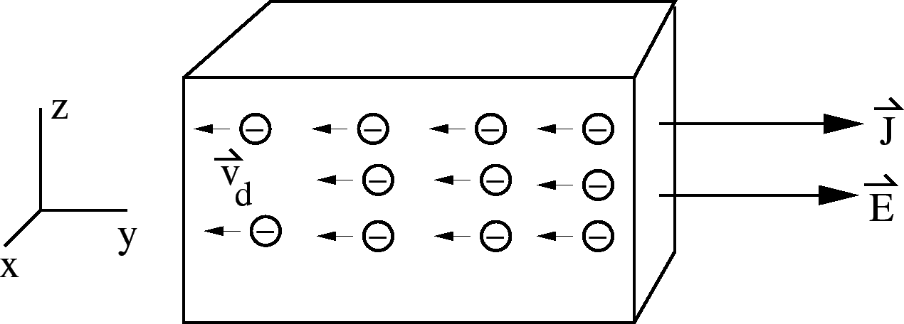
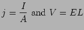
(c) Electrical Conductivity (resistivity)
Let  cross sectional area of wire,
  = length,
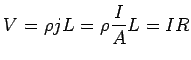
Longer wires have more resistance. Larger  means more
manuverability for electrons and less resistance. As we said
before,
means more
manuverability for electrons and less resistance. As we said
before,
 -cm.
-cm.
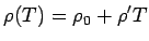
At not too low  ,
,
 (phonon scattering). As
  ,
,
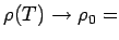 residual resistivity due to scattering of
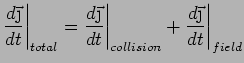
impurities. This yields Matthiessen's Rule:
residual resistivity due to scattering of
impurities. This yields Matthiessen's Rule:
 |
(1.10) |
=2.0 true in
Assumptions of the Drude model:
- (i)
- Electrons move independently under the influence of local
electric field between collisions.
- (ii)
- Collisions are instantaneous, with some unspecified but
energy-nonconserving mechanism.
- (iii)
- Collisions are random, with probability
 per unit time (no history dependence).
- (iv)
- Electrons totally thermalized to local temperature by
inelastic collisions.
DC Conductivity (
 )
)
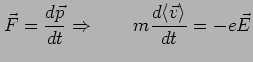
Electric current  |
(1.20) |
The minus sign is due to the negative charge of the electrons.
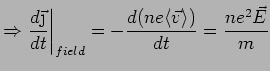
There are two contributions to

Field:
Collisions: Collisions knock electrons out of the current
flow. So we expect
 :
degrade current
:
degrade current
 |
 |
 (prob of collision (prob of collision fraction of particles affected) fraction of particles affected) |
|
| |
|
 |
|
 |
|
 |
|
 |
|
 |
|
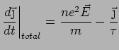
So
In a steady state with
 ,
,  must be constant:
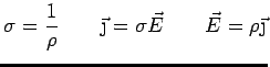
where the DC ( = constant) conductivity is given by
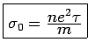 sign of
charge doesn't matter sign of
charge doesn't matter |
|
|
|
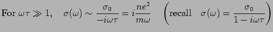
(When
 ,
,
 , i.e., the
conductivity has frequency dependence.)
, i.e., the
conductivity has frequency dependence.)
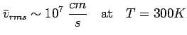
From experimental values of  and
and  , we can work out
 (see AM, table 1.2). Typically,
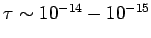 sec. at room temperature
 . At low ,
 sec and is limited by impurity scattering.
Matthiessen's rule:
sec and is limited by impurity scattering.
Matthiessen's rule:
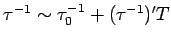 .
.
We can define a mean free path
 . How do we
estimate
. How do we
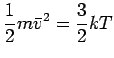
estimate  ? Drude used kinetic theory of gases and said
| |
|
 |
|
 |
|
 |
|
|
|
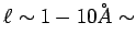 lattice spacing
or distance between ions lattice spacing
or distance between ions |
|
But this is misleading. (Should use
 cm/s)
cm/s)
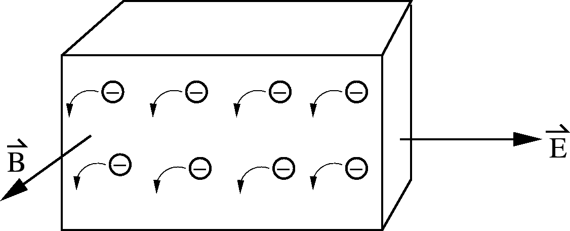
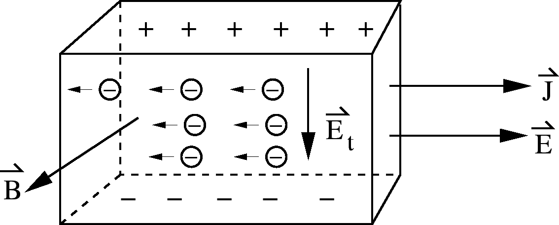
Conduction in a Magnetic Field
In the presence of a magnetic field  , an additional Lorentz
force acts on the electrons.
, an additional Lorentz
force acts on the electrons.
This leads to the Hall Effect. Consider a metal bar with
current flowing in it carried by electrons with average velocity
.
=2.5 true in
 direction.
This initially causes a downward deflection of the moving
electrons.
direction.
This initially causes a downward deflection of the moving
electrons.
=2.5 true in
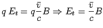
 counters the magnetic force so
that the electrons again flow in the
counters the magnetic force so
that the electrons again flow in the  direction.
=2.5 true in
 rather than
  .)
.)
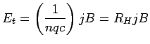
We know
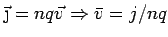
where
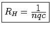 is called the Hall coefficient.
For  ,
,
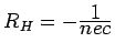
Experimentally,

 .
.
Note that because cancels the effect of the magnetic field,
we still have
 (different coords than AM). You
can check this by looking at
(different coords than AM). You
can check this by looking at
 .
Experimentally, this isn't always true. Drude model is too simple.
.
Experimentally, this isn't always true. Drude model is too simple.
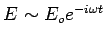
AC Conductivity

Consider an electric field that is varying in time:
The response of the electrons as well as the current will also vary
in time. This leads to a frequency dependent conductivity.
 where where |
|
|
|
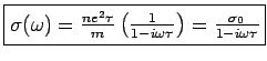
In general
will be complex, indicating that is
out of phase with  .
.
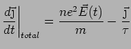
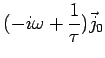
Calculate
Start with
Plug in
 and
and
 to get
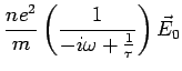
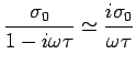
If  then then 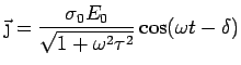 |
|
|
|
where
 .
.
=2.0 true in
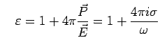
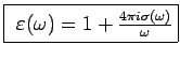
We can relate
to the frequency dependent dielectric
constant
 . Consider a piece of metal that is free-standing.
Suppose we irradiate it with electromagnetic radiation. There will
be no free current
. Consider a piece of metal that is free-standing.
Suppose we irradiate it with electromagnetic radiation. There will
be no free current
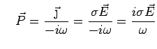
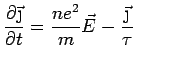
 but there will be a polarization current
because the electrons slosh back and forth:
but there will be a polarization current
because the electrons slosh back and forth:
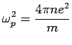
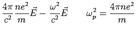
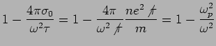
Plasma Frequency

At high frequencies (
 )
)
where
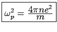 . This is called
the plasma frequency.
. This is called
the plasma frequency.
What does this mean physically?  is the characteristic
frequency for the electrons to slosh back and forth. These are
called plasma oscillations, or plasmons. AM give a simple
model of this. Imagine displacing the entire electron gas, as a
whole, through a distance
is the characteristic
frequency for the electrons to slosh back and forth. These are
called plasma oscillations, or plasmons. AM give a simple
model of this. Imagine displacing the entire electron gas, as a
whole, through a distance  with respect to the fixed positive
background of ions.
with respect to the fixed positive
background of ions.
=3.0 true in
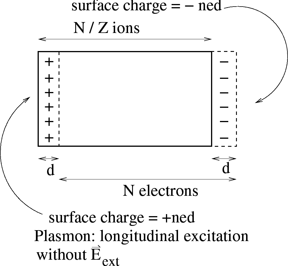
The resulting surface charge gives rise to an electric field of
magnitude
 , where
  is the charge per unit area
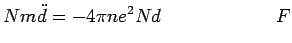
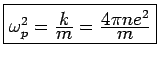
(recall Gauss' Law). The electron gas obeys the equation of motion
is the charge per unit area
(recall Gauss' Law). The electron gas obeys the equation of motion
 |
|
 |
|
| |
|
 |
|
 total number of electrons total number of electrons |
|
 |
|
 |
|
|
|
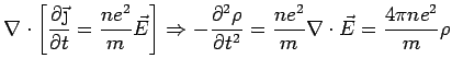
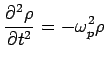
There is yet another way to derive the plasma frequency: go back to
At high frequencies
,
 we can
neglect the last term. This leaves
we can
neglect the last term. This leaves
Recall the continuity equation:
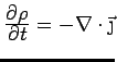 .
So
.
So
Transverse EM Waves
=2.0 true in
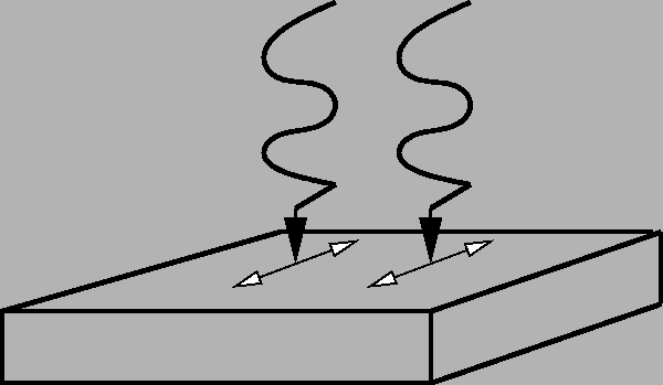
If we shine EM radiation on a metal, it will not penetrate very far
(and in fact, it will be reflected) for low frequencies because the
electrons respond quickly enough to screen it. At high frequencies,
however,
 the electrons aren't fast enough to respond
to
the electrons aren't fast enough to respond
to
 and the radiation gets through. Thus the metals become
transparent to ultraviolet light.
and the radiation gets through. Thus the metals become
transparent to ultraviolet light.
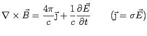
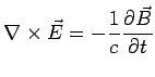
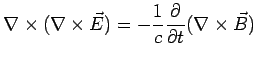
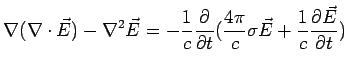
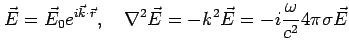
To see this mathematically, go back to Maxwell's eqns. and derive the
wave equation.
Fourier Transform w.r.t. time using
 :
:
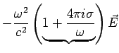
At low frequencies,
 ,
,
 and
and
 term is negligible.
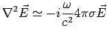
Hence
term is negligible.
Hence
Skin depth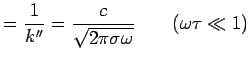 |
|
|
|
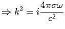
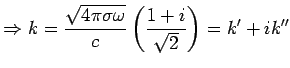
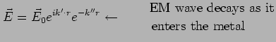
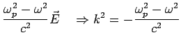
High Frequencies
For
 , this leads to exponential decay with decay length
 .
.
For
 , we get propagation and the metal becomes transparent
at a frequency
, we get propagation and the metal becomes transparent
at a frequency
 sec
sec .
.
Next: About this document ...
Previous: lecture1
Clare Yu
2004-09-30


 where
again
where
again