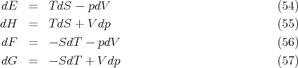
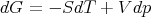
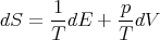
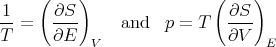
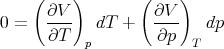
We start with the fundamental thermodynamic relation for a quasi–static infinitesimal process:

(1)

• Independent variables S and V : Equation (1) can be written

  (2)

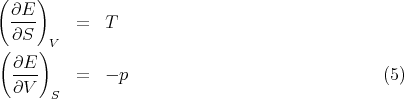
  The differentials are the independent variables. E depends on the independent parameters S and V :

  (3)

  Hence

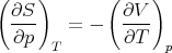
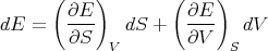  (4)

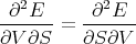
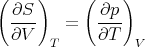
  We can write this because dE is an exact differential. Comparing (2) and (4) and matching the coefficients of dS and dV , we have

  
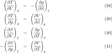
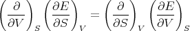
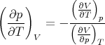
  The subscripts indicate what is held constant when the partial derivative is taken. Now note that the second derivatives of E are independent of the order of differentiation:

  (6)

  or

  (7)

  Plugging in (5), we obtain

  (8)

  This is one of Maxwell’s relations. It is a result of the fact that dE is an exact differential. It states the relation that the macroscopic parameters in eq. (1) must have in order for dE to be an exact differential.

• Independent variables S and p: Now suppose we want S and p to be the independent macroscopic parameters. To convert equation (2) to one with dS and dp, we use a trick known as a Legendre transformation.

  (9)

  or

  (10)

  Plug this into (2):

  (11)

  or

  (12)

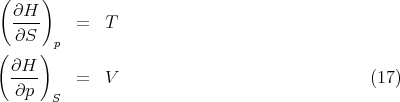
  We can write this as

  (13)

  where

  (14)

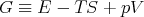
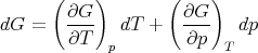
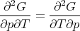
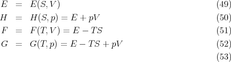
  The function H is called the “enthalpy.” It depends on the independent variables S and p:

  (15)

  The enthalpy is a state function, so we can write

  (16)

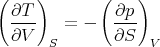
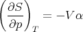
  Comparing (13) and (16), we obtain

  
  Since

  (18)

  we obtain

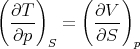  (19)

  This is another of Maxwell’s relations.

• Independent variables T and V : We now do a Legendre transformation on (2) to replace dS with dT.

  (20)

  or

  (21)

  where

  (22)

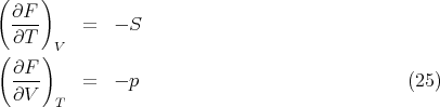
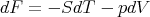
  The function F is called the “Helmholtz free energy.” When you hear physicists talk about “free energy,” they are usually referring to F. F depends on the independent variables T and V :

  (23)

  and

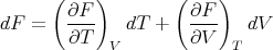  (24)

  Comparison of (21) and (24) yields

  
  Equality of the cross derivatives

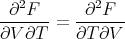  (26)

  implies

  (27)

• Independent variables T and p: In order to obtain T and p as independent variables, we perform a Legendre transformation on (2) to replace dS and dV with dT and dp:

  (28)

  or

  (29)

  where we have introduced

  (30)

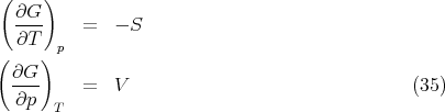
  G is called the “Gibbs free energy.” We could also write

  (31)

  or

  (32)

  G has independent variables T and p. Experimentally these are the easiest to set. So the Gibbs free energy is usually what is being dealt with experimentally.

  (33)

  and

  (34)

  Comparison of (29) and (34) yields

  
  Equality of the cross derivatives

  (36)

  implies

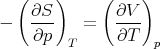  (37)

  This is also a Maxwell relation.

(42)

Notice that we can rewrite this

(43)

Since the entropy S is a state function, dS is an exact differential and we can write it as:

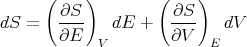(44)

Comparing coefficients of dE and dV , we find

(45)

These are relations that we derived earlier. Recall

(46)

and

(47)

Note that the conjugate pairs of variables

(48)

appear paired in (42) and when one cross multiplies the Maxwell relations. In other words the numerator on one side is conjugate to the denominator on the other side. To obtain the correct sign, note that if the two variables with respect to which one differentiates are the same variables S and V which occur as differentials in (42), then the minus sign that occurs in (42) also occurs in the Maxwell relation. Any one permutation away from these particular variables introduces a change of sign. For example, consider the Maxwell relation (39) with derivatives with respect to S and p. Switching from p to V implies one sign change with respect to the minus sign in (42); hence there is a plus sign in (39).

We also summarize the thermodynamic functions:

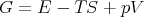(58)

At high temperatures the second term -TS is important. Water molecules have a much higher entropy in their liquid state than in their solid state. More entropy means more microstates in phase space which improves the chances of the system being in a liquid microstate. (Just like buying more lottery tickets improves your chances of winning.) The higher entropy of the liquid offsets the fact that E_water > E_ice. At low temperatures -TS is less important, so E_water > E_ice matters and the free energy for ice is lower than that of water. The transition temperature T_m between ice and water is given by

(59)

We can actually use this relation to derive an interesting relation called the Clausius–Clapeyron equation. Remember I told you that water is unusual because ice expands and because the slope of the phase boundary between ice and water is negative (dp∕dT < 0). These facts are related through the Clausius–Claperyon equation. (See Reif 8.5 for more details.)

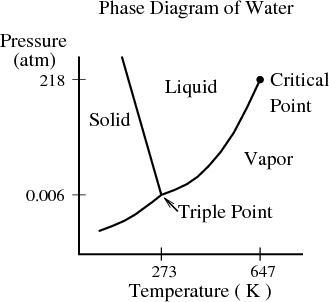
Let us consider the general case where a substance (like water) has 2 phases (like liquid and solid) with a first order transition between them. Along the phase–equilibrium line these two phases have equal Gibbs free energies:

(60)

Here g_i(T,p) = G_i(T,p)∕ν is the Gibbs free energy per mole of phase i at temperature T and pressure p. If we move a little ways along the phase boundary, then we have

(61)

Subtracting these two equations leads to the condition:

(62)

Now use (57)

(63)

where s is the molar entropy and v is the molar volume. So (62) becomes

(64)

(65)

or

(66)

where Δs = s₂ - s₁ and Δv = v₂ - v₁. This is called the Clausius–Clapeyron equation. It relates the slope of the phase boundary at a given point to the ratio of the entropy change Δs to the volume change Δv.

Let’s apply this to the water–ice transition. We know that the slope of the phase boundary dp∕dT < 0. Let phase 1 be water and let phase 2 be ice. Then Δs = s_ice - s_water < 0 since ice has less entropy than water. Putting these 2 facts together in the Clausius–Clapeyron equation implies that we must have Δv > 0. Indeed water expands on freezing and Δv = v_ice - v_water > 0. So the unusual negative slope of the melting line means that water expands on freezing. As we mentioned earlier, it also means that you can cool down a water–ice mixture by pressurizing it and following the coexistence curve, i.e., the melting line or phase boundary.

Another example is ³He which also has a melting line with a negative slope. The fact that dp∕dT < 0 means that if you increase the pressure on a mixture of liquid and solid ³He, the temperature will drop. This is the principle behind cooling with a Pomeranchuk cell. Unlike the case of water where ice floats because it is less dense, solid ³He sinks because it is more dense than liquid ³He. The Clausius–Clapeyron equation then implies that Δs = s _solid - s_liquid > 0, i.e., solid ³He has more entropy than liquid ³He! How can this be? It turns out that it is spin entropy. A ³He atom is a fermion with a nuclear spin 1/2. The atoms in liquid ³He roam around and their wavefunctions overlap, so that liquid ³He has a Fermi sea just like electrons do. The Fermi energy is lower if the ³He atoms can pair up with opposite spins so that two ³He atoms can occupy each translational energy state. However, in solid liquid ³He, the atoms are centered on lattice sites and the wavefunctions do not overlap much. So the spins on different atoms in the solid are not correlated and the spin entropy is ~ R ln 2 which is much larger than in the liquid.

Now back to the general case. Since there is an entropy change associated with the phase transformation from phase 1 to phase 2, heat must be absorbed (or emitted). The “latent heat of transformation” L₁₂ is defined as the heat absorbed when a given amount of phase 1 is transformed to phase 2. For example, to melt a solid, you dump heat into it until it reaches the melting temperature. When it reaches the melting temperature, its temperature stays at T_m even though you continue to dump in heat. It uses the absorbed heat to transform the solid into liquid. This heat is the latent heat L₁₂. Since the process takes place at the constant temperature T_m, the corresponding entropy change is simply

(67)

Thus the Clausius–Clapeyron equation (66) can be written

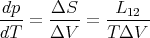(68)

If V refers to the molar volume, then L₁₂ is the latent heat per mole; if V refers to the volume per gram, then L₁₂ is the latent heat per gram. In most substances, the latent heat is used to melt the solid into a liquid. However, if you put heat into liquid ³He when it is on the melting line, it will form solid because solid ³He has more entropy than liquid ³He.

(69)

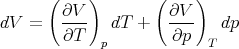
We want to replace dS with dV . So we regard the entropy as a function of the independent variables V and T:

(70)

dS is an exact differential:

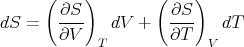(71)

Since we are interested in (∂E∕∂V )_T at constant temperature, dT = 0 and

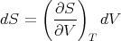(72)

Now use the Maxwell relation (40):

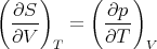(73)

So we have

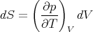(74)

and

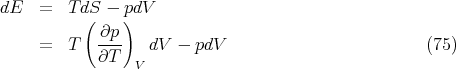
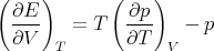(76)

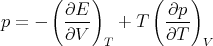
Let’s take a moment to consider what this means physically. We know that gas cools when it expands, and that the pressure rises when it is heated. There must be some connection between these two phenomena. Microscopically we can think of the kinetic energy of the gas molecules. Macroscopically, eq. (76) gives the relation. If we hold the volume fixed and increase the temperature, the pressure rises at a rate (∂p∕∂T)_V . Related to that fact is this: if we increase the volume, the gas will cool unless we pour some heat in to maintain the temperature, and (∂E∕∂V )_T dV tells us the amount of heat needed to maintain the temperature. (Notice that for an ideal gas ∂E∕∂V = 0.) Equation (76) expresses the fundamental relation between these two effects. Notice that we didn’t need to know the microscopic interactions between the gas particles in order to deduce the relationship between the amount of heat needed to maintain a constant temperature when the gas expands, and the pressure change when the gas is heated. That’s what thermodynamics does; it gives us relationships between macroscopic quantities without having to know about microscopics.

Aside: Notice that

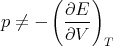(77)

as one might expect. Rather

(78)

However,

(79)

implies that

(80)

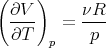
It matters what is kept constant! Recall from (25) that

(81)

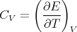
The heat capacity at constant volume is given by

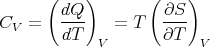(82)

and the heat capacity at constant pressure is

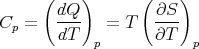(83)

Let us consider the independent variables as T and p. Then S = S(T,p) and

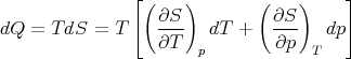(84)

Using (83), we have

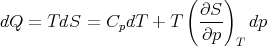(85)

At constant pressure, dp = 0 and we obtain (83). But to calculate C_V , we see from (82) that T and V are the independent variables. So we plug

(86)

into (85) to obtain

(87)

Constant V means that dV = 0 and so

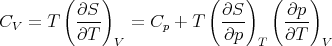(88)

This is a relation between C_V and C_p but it involves derivatives which are not easily measured. However we can use Maxwell’s relations to write this relation in terms of quantities that are measurable. In particular (41) is

(89)

The change of volume with temperature at constant pressure is related to the “volume coefficient of expansion” α (sometimes called the coefficient of thermal expansion):

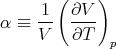(90)

Thus

(91)

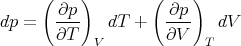
The derivative (∂p∕∂T)_V is also not easy to measure since measurements at constant volume are difficult. It is easier to control T and p. So let’s write

(92)

For constant volume dV = 0 and

(93)

we can rearrange this get an expression for dp∕dT:

(94)

Aside: This is an example of the general relation proved in Appendix 9. If we have 3 variables x, y, and z, two of which are independent, then we can write, for example,

(95)

and

(96)

At constant z we have dz = 0 and

(97)

Thus

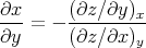(98)

or, since z was kept constant

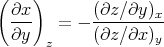(99)

This sort of relation between partial derivatives is used extensively in thermodynamics.

Returning to (94), we note that the numerator is related to the expansion coefficient α. The denominator measures the change in the volume of the substance with increasing pressure at constant temperature. The change of the volume will be negative, since the volume decreases with increasing pressure. We can define the “isothermal compressibility” of the substance:

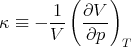(100)

The compressibility is a measure of how squishy the substance is. Hence (94) becomes

(101)

Plugging (91) and (101) into (88) yields

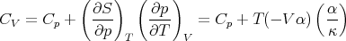(102)

or

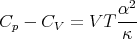(103)

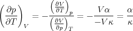
Let’s test this formula on the simple case of an ideal gas. We start with the equation of state:

(104)

We need to calculate the expansion coefficient. For constant p

(105)

Hence

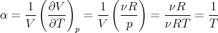(106)

Next we calculate the compressibility κ. At constant temperature the equation of state yields

(107)

Hence

(108)

and

(109)

Thus (103) becomes

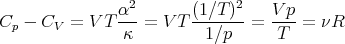(110)

or, per mole,

(111)

which agrees with our previous result.

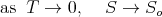(112)

This implies that the derivative (∂S∕∂T) remains finite as T → 0. In other words, it does not go to infinity. (Technically speaking, the derivatives appearing in (82) and (83) remain finite as T goes to 0.) So one can conclude that the heat capacity goes to 0 as T → 0:

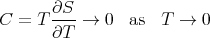(113)

or more precisely,

(114)

The fact that the heat capacity goes to 0 at zero temperature merely reflects the fact that the system settles into its ground state as T → 0. If we recall that

(115)

then reducing the temperature further will not change the energy since the energy has bottomed out. Notice that we need C_V (T) → 0 as T → 0 in order to guarantee proper convergence of the integral in

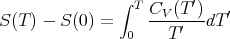(116)

The entropy difference on the left must be finite, so the integral must also be finite.