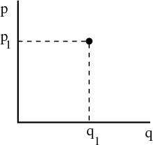
In classical mechanics if we have a single particle in one dimension then we can describe the system completely by specifying the position coordinate q and the momentum coordinate p. We can represent this graphically by labeling one axis with q and one axis with p:
We call the space spanned by p and q “phase space.” It’s the space in which the point
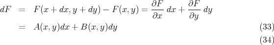
(q1,p1) exists. If our system has N particles and exists in 3D, then we must provide  i and
i and  i
for all N particles. Since
i
for all N particles. Since  and
and  are each 3 dimensional vectors, if we want to represent the
system as a point in phase space, we need 6N axes. In other words phase space is 6N
dimensional. The coordinates of the point representing the system in phase space are
(qx1,qx2,...,qzN,px1,...pzN).
are each 3 dimensional vectors, if we want to represent the
system as a point in phase space, we need 6N axes. In other words phase space is 6N
dimensional. The coordinates of the point representing the system in phase space are
(qx1,qx2,...,qzN,px1,...pzN).
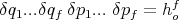
Spatial coordinates and momenta are continuous variables. To obtain a countable number of states, we divide phase space into little boxes or cells. For our one particle in 1D example, the volume of one of these cells is
 | (1) |
where ho is some small constant having the dimensions of angular momentum. The state of the system can then be specified by stating that its coordinate lies in some interval between q and q + δq and between p and p + δp. For our N particle system, f = 3N spatial coordinates and f momentum coordinates are required to specify the system. So the volume of a cell in phase space is
 | (2) |
Each cell in phase space corresponding to a state of the system can be labeled with some number. The state of a system is provided by specifying the number of the cell in phase space within which the system is located.
One microscopic state or microstate of the system of N particles is defined by specifying all the coordinates and momenta of each particle. An N particle system at any instant of time is specified by only one point in a 6N dimensional phase space and the corresponding microstate by the numerical label of the cell in which this point is located. As the system evolves in time, the coordinates of the particles change, and the N particle system follows some trajectory in this 6N dimensional phase space.
A macroscopic state or macrostate of the system is determined by only a few macroscopic parameters such as temperature, energy, pressure, magnetization, etc. Note that a macrostate contains much less information about a system than a microstate. So a given macrostate can correspond to any one of a large number of microstates.
How would quantum mechanics be used to describe a system? Any system of N interacting particles can be described by a wavefunction
 | (3) |
where the qi are the appropriate “coordinates” for the N particles. The coordinates include both spin and space coordinates for each particle in the system. A particular state (or a particular wavefunction) is then specified by providing the values of a set of quantum numbers {n}. This set of quantum numbers can be regarded as labelling this state. Different values of the quantum numbers correspond to different states. For simplicity let’s just label the states by some index r, where r = 1, 2, 3, ... The index r then labels the different microstates. In quantum mechanics, ho is replaced by Planck’s constant h.
Thus both classical and quantum mechanics lead to a countable number of microstates for an N particle system.
This concept, and the term enemble, were introduced by J. W. Gibbs, an American physicist around the turn of the 20th century.
Another basic approach to statistical mechanics, proposed by Boltzmann and Maxwell, is known as the ergodic hypothesis. According to this view, the macroscopic properties of a system represent averages taken over the microstates traversed by a single system in the course of time. It is supposed that systems traverse all the possible microstates fast enough that the time averages are identical with the averages taken over a large collection of identical and independent systems, i.e., an ensemble. This is the idea behind Monte Carlo simulations.
An isolated system in equilibrium is equally likely to be in any of its accessible states. In other words if phase space is subdivided into small cells of equal size, then an isolated system in equilibrium is equally likely to be in any of its accessible cells.
Certainly this seems reasonable. There is no reason for one microstate to be preferred over another, as long as each microstate is consistent with the macroscopic parameters. There are also more rigorous reasons to accept this postulate. It’s a consequence of Liouville’s theorem (see Appendix 13 of Reif) that if a representative ensemble of such isolated systems are distributed uniformly over their accessible states at any one time, then they will remain uniformly distributed over these states forever.
One can think of the accessible states as the “options” that a system has available to it. Lots of accessible states means lots of possible microstates that the system can be in.
What if an isolated system is not equally likely to be found in any of the states accessible to it? Then it is not in equilibrium. But it will approach equilibrium. The system will make transitions between all its various accessible states as a result of interactions between its constituent particles. Once the system is equally likely to be in any of its accessible states, it will be in equilibrium, and it will stay that way forever (at least as long as it is isolated). The idea that a nonequilibrium system will approach equilibrium is a consequence of the H theorem (Appendix 12 in Reif). If we think in terms of an ensemble of systems distributed over the points in phase space in some arbitrary way, then the ensemble will evolve slowly in time until phase space is uniformly occupied. The characteristic time associated with attaining equilibrium is called the “relaxation time.” The magnitude of the relaxation time depends on the details of the system. The relaxation time can range from less than a microsecond to longer than the age of the universe (e.g., glass). Indeed the glass transition is a good example of a system falling out of equilibrium because the experimenter cannot wait long enough for the system to equilibrate. Calculating the rate of relaxation toward equilibrium is quite difficult, but once equilibrium is reached and things become time–independent, the calculations become quite straightforward. For example, many of the properties of the early universe have been calculated using the assumption that things were in equilibrium.
 | (4) |
To calculate the mean value of the parameter y of the system, we simply take the average over the systems in the ensemble; i.e.,
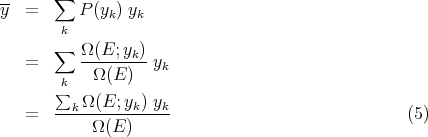
 | (6) |
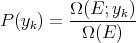
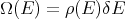
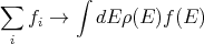
where ρ(E) is the “density of states”. (Your book writes it as w(E).) The density of states is a characteristic property of the system which measures the number of states per unit energy range. For example one could have the number of states per eV. The density of states is an important concept in systems with many particles. For example in a simple metal where electrons conduct electric current, the density of electron states near the Fermi energy determines how good a conductor the metal is. If the density of states is high, then the metal is a good conductor because the electrons near the Fermi energy will have a lot of empty states to choose from when they hop. If ρ(E) is small, then the metal is a poor conductor because the electrons will not have many empty states to hop to. The density of states is often useful in converting sums into integrals over energy:
 | (7) |
 | (8) |
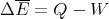
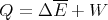
Heat is energy transfer. The heat can be positive or negative. -Q is the heat given off by a system; Q is the heat absorbed by the system. Since the total energy is unchanged
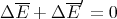 | (9) |
or
 | (10) |
or
 | (11) |
This is just conservation of energy.
 | (12) |
The macroscopic work W done by the system is the negative of  :
:
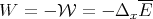 | (13) |
Conservation of energy dictates that
 | (14) |
or
 | (15) |
Doing work on a system changes the positions of the energy levels and the occupation of different states.
 | (16) |
(We should keep the entropy fixed in this derivative.)
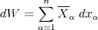
We can make this more formal. When we say “macroscopic work,” we mean more than pdV or Fdx where F is a force. Let the energy of some microstate r depend on external parameters x1,...,xn.
 | (17) |
Then when the parameters are changed by infinitesimal amounts, the corresponding change in energy is
 | (18) |
The work dW done by the system when it remains in this particular state r is then defined as
 | (19) |
where
 | (20) |
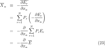
This is called the “generalized force” conjugate to the external parameter xα in the state r. Note that if xα denotes a distance, then Xα simply is an ordinary force.
Consider an ensemble of similar systems. If the external parameters are changed quasi–statically so that the system remains in equilibrium at all times, then we can calculate the mean value averaged over all accessible states r
 | (21) |
where
 | (22) |
is the mean generalized force conjugate to xα. Note that
Examples
 | (24) |
where x is the linear dimension and Fx is the ordinary force in the x direction.
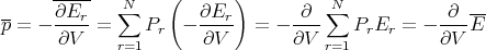
 | (25) |
where p is the average pressure and V is volume. We wrote down the expression for pressure before, but now we can be more precise. The pressure is the generalized force associated with changes in volume.
 | (26) |
or
 | (27) |
where E is the macroscopic energy and V is the volume.
Your book talks about quasi–static processes in which the process occurs so slowly that the system can be regarded as being in equilibrium throughout. For example, the piston can be moved so slowly that the gas is always arbitrarily close to equilibrium as its volume is being changed. In this case the mean pressure has a well–defined meaning. If the volume is changed by an infinitesimal amount dV , then the work done is
 | (28) |
If the volume is changed from an initial volume V i to a final volume V f, then the macroscopic amount of work done is given by
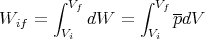 | (29) |
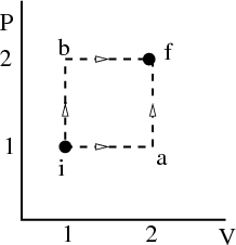
The work done is the area under the pressure curve between V i and V f in the P-V diagram.
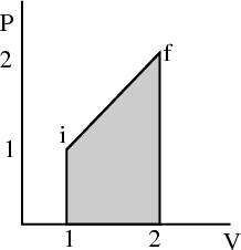
This integral depends on the path taken from the initial to the final volume. It is not path independent. For example, in the figure, the area under the path i → b → f is twice the area under the path i → a → f, even though the endpoints of both paths are the same.
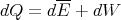
So dW is not an exact differential. (Recall in electromagnetism, the potential difference is path independent.) dW is not the difference of 2 numbers referring to 2 neighboring macrostates; rather it is characteristic of the process of going from state i to state f. Similarly the infinitesimal amount of heat dQ absorbed by the system in some process is also not an exact differential and in general, will depend on how the process occurs.
 | (30) |
This is the first law of thermodynamics. If we write
 | (31) |
then we can view the heat Q as the mean energy change not due to a change in the external parameters. For infinitesimal changes, we can write
 | (32) |
Note that dE is an exact differential. The change in the mean energy is independent of the path taken between the initial and final states. The energy is characteristic of the state, not of the process in getting to that state.
For example, suppose we push a cart over a bumpy road to the top of a hill. Let us suppose there are 2 roads to the top of the hill. How much work we do and how much is lost to friction and heat depends on which road we take and how long the road is. However, at the end of our journey at the top of the hill, the (potential) energy is independent of the road we chose. This is why dQ and dW are inexact differentials but dE is an exact differential.
Note that if dQ = 0, dE = -dW is an exact differential. So if Q = 0, then ΔEif = -Wif. On the other hand, if dW = 0, dE = dQ and dQ is an exact differential. So if W = 0, ΔEif = Qif.
 | (35) |
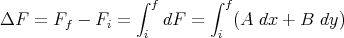
Note that the integral of an exact differential depends only on the endpoints (initial and final points) and not on the path of integration.
However, not every function is an exact differential. Consider
 | (36) |
It is not guaranteed that there will exist a function G(x,y) such that
 | (37) |
That is, it is not always true that
 | (38) |
is independent of the path between the endpoints. The integral may depend on the path of integration. As an example, consider
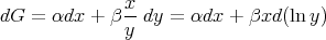 | (39) |
It is easy to show that
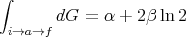 | (40) |
and
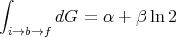 | (41) |
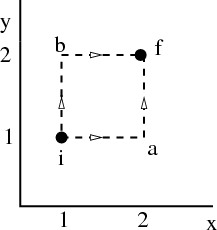
Note however that if
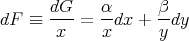 | (42) |
then dF is an exact differential with
 | (43) |
and
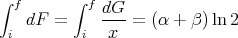 | (44) |
independent of path. The factor 1∕x is called an integrating factor for dG.