(References: Kerson Huang, Statistical Mechanics, Wiley and Sons (1963) and Colin Thompson, Mathematical Statistical Mechanics, Princeton Univ. Press (1972)).
One of the simplest and most famous models of an interacting system is the Ising model. The Ising model was first proposed in Ising’s Ph.D thesis and appears in his 1925 paper based on his thesis (E. Ising, Z. Phys. 31, 253 (1925).) In his paper Ising gives credit to his advisor Wilhelm Lenz for inventing the model, but everyone calls it the Ising model. The model was originally proposed as a model for ferromagnetism. Ising was very disappointed that the model did not exhibit ferromagnetism in one dimension, and he gave arguments as to why the model would not exhibit ferromagnetism in two and three dimensions. We now know that the model does have a ferromagnetic transition in two and higher dimensions. A major breakthrough came in 1941 when Kramers and Wannier gave a matrix formulation of the problem. In 1944 Lars Onsager gave a complete solution of the problem in zero magnetic field. This was the first nontrivial demonstration of the existence of a phase transition from the partition function alone.
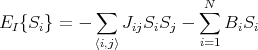
Consider a lattice of N sites with a spin S on each site. Each spin can take one of two possible values: +1 for spin up and -1 for spin down. There are a total of 2N possible configurations of the system. A configuration is specified by the orientations of the spins on all N sites: {Si}. Si is the spin on the ith lattice site. The interaction energy is defined to be
|
| (1) |
where the subscript I represents the Ising model. A factor of 2 has been absorbed into Jij and
we set gμB = 1 in the last term. ⟨i,j⟩ means nearest neighbor pairs of spins. So ⟨i,j⟩ is the
same as ⟨j,i⟩. Jij is the exchange constant; it sets the energy scale. For simplicity, one
sets Jij equal to a constant J. If J > 0, then the spins want to be aligned parallel
to one another, and we say that the interaction is ferromagnetic. If J < 0, then
the spins want to be antiparallel to one another, and we say that the interaction is
antiferromagnetic. If Jij is a random number and can either be positive or negative, then we
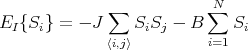
have what is called a spin glass. For simplicity we will set Jij = J > 0 and study the
ferromagnetic Ising model. The last term represents the coupling of the spins to an
external magnetic field B. The spins are assumed to lie along the z-axis as is the
magnetic field  = Bẑ. The spins lower their energy by aligning parallel to the field.
I put Bi to indicate the possibility that the field could vary from spin to spin. If
the field Bi is random, this is called the random field Ising model. We will assume
a constant uniform magnetic field so that Bi = B > 0. So the interaction energy
becomes
= Bẑ. The spins lower their energy by aligning parallel to the field.
I put Bi to indicate the possibility that the field could vary from spin to spin. If
the field Bi is random, this is called the random field Ising model. We will assume
a constant uniform magnetic field so that Bi = B > 0. So the interaction energy
becomes
 | (2) |
The partition function is given by
 | (3) |
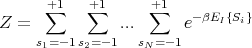
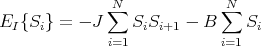
Let us consider the one-dimensional Ising model where N spins are on a chain. We will impose periodic boundary conditions so the spins are on a ring. Each spin only interacts with its neighbors on either side and with the external magnetic field B. Then we can write
 | (4) |
The periodic boundary condition means that
 | (5) |
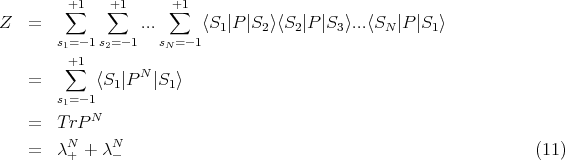
The partition function is
![[ ]
+∑1 +∑1 +∑1 N∑
Z = ... exp β (JSiSi+1 + BSi )
s1=- 1s2= -1 sN= -1 i=1](lecture186x.png) | (6) |
Kramers and Wannier (Phys. Rev. 60, 252 (1941)) showed that the partition function can be expressed in terms of matrices:
![+∑1 +∑1 +∑1 [ ∑N ( ) ]
Z = ... exp β JSiSi+1 + 1B (Si + Si+1)
s1= -1s2=-1 sN =-1 i=1 2](lecture187x.png) | (7) |
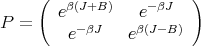
This is a product of 2 × 2 matrices. To see this, let the matrix P be defined such that its matrix elements are given by
![{ [ ]}
⟨S |P |S′⟩ = exp β JSS ′ + 1B (S + S ′)
2](lecture188x.png) | (8) |
where S and S′ may independently take on the values ±1. Here is a list of all the matrix elements:
![⟨+1 |P | + 1⟩ = exp[β(J + B )]
⟨- 1|P | - 1⟩ = exp[β(J - B )]
⟨+1 |P | - 1⟩ = ⟨+1 |P | - 1⟩ = exp [- βJ ] (9)](lecture189x.png)
 | (10) |
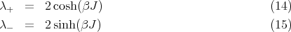
With these definitions, we can write the partition function in the form
 | (12) |
Solving this quadratic equation for λ gives
![[ ∘ -----------------------------]
λ± = eβJ cosh(βB ) ± cosh2(βB ) - 2e-2βJ sinh(2βJ )](lecture1813x.png) | (13) |
When B = 0,
 < 1 and write the Helmholtz free energy per spin:
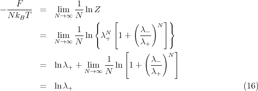
![F-- = - kBT--ln Z = - kBT lnλ+
N N [ ∘ -----------------------------]
= - J - k T ln cosh(βB ) + cosh2(βB ) - 2e -2βJ sinh(2βJ ) (17)
B](lecture1817x.png)
![M--
m = N
1 ∂ ln Z
= ----------
βN ∂B
1-∂F--
= - N ∂B
sinh(βB )
= ∘------------------------------- (18)
cosh2(βB ) - 2e-2βJ sinh(2βJ )]](lecture1818x.png)
The method of transfer matrices can be generalized to two and higher dimensions, though the matrices become much larger. For example, in two dimensions on an m × m square lattice, the matrices are 2m × 2m. In 1944, Onsager solved the two dimensional Ising model exactly for the zero field case, and found a finite temperature ferromagnetic phase transition. This is famous and is known as the Onsager solution of the 2D Ising model. No one has found an exact solution for the three dimensional Ising model.
 i -
i - j|)
with
j|)
with
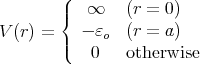 | (19) |
where a is the lattice spacing. The occupation ni of a lattice site i is given by
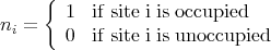 | (20) |
The interaction energy is
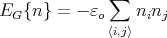 | (21) |
We can map this into the Ising model by letting spin-up denote an occupied site and letting spin-down denote an unoccupied site. Mathematically, we write
 | (22) |
So Si = 1 means site i is occupied and Si = -1 means site i is unoccupied. One can then map the lattice gas model into Ising model. For example, by comparing the partition functions, it turns out that ϵo = 4J.
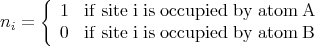 | (23) |
There are interaction energies between nearest neighbor sites: εAA, εBB and εAB. One can map the binary alloy model into the lattice gas model and the Ising model.
Quantum mechanically, the values of Sz are discretized. So Ising spins correspond to
⟨Sz⟩ = ±1∕2.  =
=  ∕2 where
  are the Pauli spin matrices.
We have already mentioned that the Ising model can be considered in higher dimensions. Another variation of the Ising model is to consider other types of lattices. For example in two dimensions, we could have a triangular lattice. In three dimensions there are a wide variety of lattice structures that could be considered. Or one could throw away the lattice and have randomly placed sites to make a type of spin glass.
Other variations center around the form of the interaction. For example, we can allow the nearest neighbor interactions to be antiferromagnetic. Or we can allow the interactions to extend over a longer range to include next nearest-neighbors or even farther, e.g., infinite range. The interaction is contained in the exchange constant Jij. So one could have something like
 | (24) |
where n = 1 is the Coulomb interaction and n = 3 is similar to a dipolar interaction. Another interaction is the RKKY interaction. RKKY stands for Ruderman-Kittel-Kasuya-Yosida. The RKKY interaction has the form
 | (26) |
Typically, Jij is chosen from a distribution P(J) centered at J = 0. For example, Jij = ±J where J is a positive constant, and there is an equal probability of choosing the plus or minus sign. Another possibility is to have P(J) be a Gaussian distribution centered at J = 0. Obviously the ground state of a such a system will be disordered, but a phase transition from a paramagnetic phase at high temperatures to a frozen spin configuration is possible.
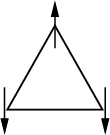
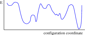
One concept that is associated with spin glasses is “frustration.” The idea is best illustrated by considering an equilateral triangle with a spin on each vertex. Suppose the interaction between nearest neighbor spins is antiferromagnetic so that a spin wants to point opposite from its neighbors. There is no way all the spins on the triangle can be satisfied. This is an example of frustration. Frustration occurs when there is no spin configuration where all the spins have their lowest possible interaction energy. In a spin glass, there is a great deal of frustration. As a result there is no clear ground state configuration. One can associate an energy landscape with the energies of different spin configurations. Valleys correspond to low energy configurations and mountains to high energy configurations. The landscape exists in the space of spin configurations. So to go from one valley to another, the system must climb out of the first valley by going through some high energy configurations and then descend into the second valley by passing through configurations with decreasing energy.
Spin glasses are often used to model interacting systems with randomness. They were originally proposed to explain metals with magnetic impurities and were thought to be a simple model of a glass. Spin glass models have a wide range of applications, e.g., they have been used to model the brain and were the basis of neural networks and models of memory.
Reference: D. P. Landau and K. Binder, A Guide to Monte Carlo Simulations in Statistical Physics, Cambridge Univ. Press (2000).
As one can see, analytic solutions to spin systems can be difficult to obtain. So one often resorts to computer simulations, of which Monte Carlo is one of the most popular. Monte Carlo simulations are used widely in physics, e.g., condensed matter physics, astrophysics, high energy physics, etc. Typically in Monte Carlo simulations, one evolves the system in time. The idea is to visit a large number of configurations in order to do statistical sampling. For a spin system we would want to obtain average values of thermodynamic quantities such as magnetization, energy, etc. More generally, Monte Carlo is an approach to computer simulations in which an event A occurs with a certain probability PA where 0 ≤ PA ≤ 1. In practice, during each time step, a random number x is generated with uniform probability between 0 and 1. If x ≤ PA, event A occurs; if x > PA, event A does not occur. Monte Carlo is also able to handle cases where multiple outcomes are possible. For example, suppose there are three possibilities so that either event A can occur with probability PA or event B can occur with probability PB or neither occurs. Then if x ≤ PA, A occurs; if PA < x ≤ (PA + PB), B occurs; and if (PA + PB) < x ≤ 1, neither occurs.
The Metropolis algorithm (Metropolis et al., J. Chem. Phys. 21, 1087 (1953)) is a classic Monte Carlo method. Typically, configurations are generated from a previous state using a transition probability which depends on the energy difference ΔE between the initial and final states. For relaxational models, such as the (stochastic) Ising model, the probability obeys a master equation of the form:
![∂P (t) ∑
--n----= [- Pn(t)Wn →m + Pm (t)Wm →n]
∂t n⁄=m](lecture1834x.png) | (27) |
where Pn(t) is the probability of the system being in state n at time t, and Wn→m is the transition rate from state n to state m. This is an example of a master equation. Master equations are found in a wide variety of contexts, including physics, biology (signaling networks), economics, etc.
In equilibrium ∂Pn(t)∕∂t = 0 and the two terms on the right hand side must be equal. The result is known as ‘detailed balance’:
 | (28) |
Loosely speaking, this says that the flux going one way has to equal the flux going the other way. Classically, the probability is the Boltzmann probability:
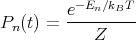 | (29) |
The problem with this is that we do not know what the denominator Z is. We can get around this by generating a Markov chain of states, i.e., generate each new state directly from the preceding state. If we produce the nth state from the mth state, the relative probability is given by the ratio
 .
.
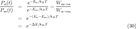
Any transition rate which satisfies detailed balance is acceptable. Historically the first choice of a transition rate used in statistical physics was the Metropolis form:
 | (31) |
Here is a recipe on how to implement the Metropolis algorithm on a spin system:
 , flip the spin.
The random number r is chosen from a uniform distribution. The states are generated with a Boltzmann probability. The desired average of some quantity A is given by ⟨A⟩ = ∑ nPnAn. In the simulation, this just becomes the arithmetic average over the entire sample of states visited. If a spin flip is rejected, the old state is counted again for the sake of averaging. Every spin in the system is given a chance to flip. One pass through the lattice is called a “Monte Carlo step/site” (MCS). This is the unit of time in the simulation.
For purposes of a spin model, it is easier to calculate ΔE if we write
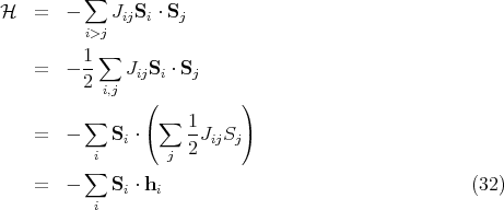
 | (33) |
To find the change in energy, we would do a trial flip of Si and easily calculate the new energy if we know the local field hi. If we accept the flip, then we have to update the local fields of the neighboring spins.
As we said before, Monte Carlo simulations are used widely in physics as well as other fields such as chemistry, biology, engineering, finance, etc.