that is related to the spin
by
that is related to the spin
by
Consider a solid consisting of N identical atoms arranged in a regular lattice. Each atom
has a net electronic spin S and a magnetic moment that is related to the spin
by
 | (1) |
where g is the g-factor and μo is the Bohr magneton. In the presence of an externally applied
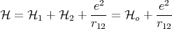
magnetic field Ho along the z direction, the Hamiltonian  o is given by
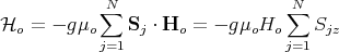 | (2) |
In addition, each atom can interact with its neighbors. In the past we ignored interactions and assumed that the spins were noninteracting. This is ok as long as kBT ≫ the interaction energy. In this case, well-localized spins should obey Curie’s law, χ ~ 1∕T, far from saturation and the magnetization M should vanish as Ho → 0. This is how a paramagnet behaves.
However, if the interaction between spins  kBT, magnetic ordering may occur. We can
think of this as being due to an effective magnetic field produced at a given site by its
neighbors. For example, suppose a given electron is ↑. If it produces a field at a neighboring
site parallel to itself, then the neighbor will also tend to be polarized ↑: in fact, we would
expect all ↑ spins or all ↓ spins in the ground state. This is a ferromagnet – it has
“spontaneous magnetization” even when Ho = 0. Ferromagnets are bar magnets and stick
to your refrigerator door. If, on the other hand, the field produced is antiparallel
to the spin, we expect to get ↑↓↑↓ .... This is an antiferromagnet and has zero net
magnetization.
kBT, magnetic ordering may occur. We can
think of this as being due to an effective magnetic field produced at a given site by its
neighbors. For example, suppose a given electron is ↑. If it produces a field at a neighboring
site parallel to itself, then the neighbor will also tend to be polarized ↑: in fact, we would
expect all ↑ spins or all ↓ spins in the ground state. This is a ferromagnet – it has
“spontaneous magnetization” even when Ho = 0. Ferromagnets are bar magnets and stick
to your refrigerator door. If, on the other hand, the field produced is antiparallel
to the spin, we expect to get ↑↓↑↓ .... This is an antiferromagnet and has zero net
magnetization.
All forms of magnetic ordering disappear as the substance is heated: typical transition temperatures are of order 100 to 1000 K. The temperature at which the spontaneous magnetization disappears is called the Curie temperature (TC) for a ferromagnet. The ordering temperature for an antiferromagnet (AF) is called the Néel temperature (TN).
Origin of the Ordering Field: Our first guess of the dominant magnetic interactions would be magnetic dipole-dipole interactions. But the strength of nearest neighbor dipole-dipole interactions is of order 1 K which is much smaller than the transition temperature (TC) for a ferromagnet. (See Reif page 429 for more details of this estimate.) So dipolar interactions cannot account for magnetic ordering.
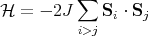
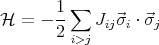
The origin of the ordering field is a quantum mechanical exchange effect. The derivation is given in the appendix and you will see it in the second quarter of quantum mechanics. Let me try to explain the physics behind the exchange effect. Basically the Coulomb interaction between two spins depends on whether the spins form a singlet or a triplet. A triplet state is antisymmetric in real space while the singlet state has a symmetric wavefunction in real space. So the electrons stay out of each others way more when they are in the triplet state. As a result, the Coulomb interaction between two electrons is less when they are in a triplet state than when they are in a singlet state. So the interaction energy depends on the relative orientations of the spins. This can be generalized so the spins don’t have to belong to electrons and the spins need not be spin-1/2. This interaction between spins is called the exchange interaction and the Hamiltonian can be written as
 | (3) |
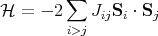
This is known as the Heisenberg Hamiltonian. We put i > j in the sum to prevent double counting. Jij is called an exchange constant. Since it depends on the overlap of wavefunctions, it falls off rapidly as the distance between the spins increases. Often Jij is taken to be non-zero only between nearest neighbor spins. If we take Jij = J, then
 | (4) |
Notice that if J > 0, then the spins lower their energy by aligning parallel to each other. If J < 0, the spins are anti-parallel in their lowest energy spin configuration. (In a spin glass, Jij is a random number that is different for each pair i and j.)
The spins need not have S = 1∕2. For example, if there is both spin and orbital angular momentum (S and L), then Ji = Li + Si is the relevant “spin” vector. Ji is the total angular momentum of the ith atom.
A simpler Hamiltonian can be obtained by just considering the z components of the spins. This is called the Ising model.
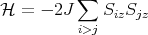 | (5) |
For S = 1∕2, Sz can take only 2 values: +1/2 or -1∕2.
Magnetic systems are not only important in their own right, but also because they are simple examples of interacting systems and can represent other types of systems, e.g., a system of neurons.
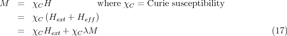
This is a prototype for mean field theories and second order phase transitions. In 1907 Pierre Weiss proposed an effective field approximation in which he considered only one magnetic atom and replaced its interaction with the remainder of the crystal by an effective magnetic field Heff. We can extract the single atom Hamiltonian from the Heisenberg Hamiltonian:
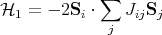 | (6) |
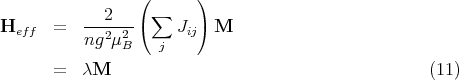
We now wish to replace the interactions with other spins by an effective magnetic field Heff so
that 1 has the form
 | (7) |
where
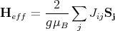 | (8) |
In the spirit of the Weiss approximation, we then assume that each Sj can be replaced by its average value ⟨Sj⟩ = ⟨S⟩
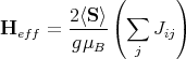 | (9) |
By assumption, all magnetic atoms are identical and equivalent. This implies that ⟨S⟩ is related to the magnetization of the crystal by
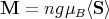 | (10) |
where n is the number of spins per unit volume.
 | (12) |
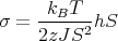
If there are only nearest-neighbor interactions, ∑ jJij = zJ where z is the number of nearest neighbors, i.e., the coordination number. Then
 | (13) |
If there is an external field Hext, then the total field acting on the ith spin is
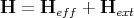 | (14) |
Since M is a paramagnetic function of H:
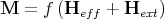 | (15) |
where
 | (16) |
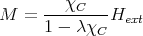
We can solve these two equations self-consistently for M. Let’s do some simple examples of this.
 | (18) |
Since χ = ∂M∕∂Hext, we get
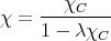 | (19) |
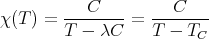
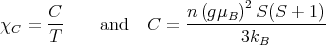
Putting χC = C∕T, where C is the Curie constant, gives the Curie-Weiss Law:
 | (20) |
where TC = λC. This reduces to the Curie law χ C∕T for T ≫ TC, but as we approach
TC from above, the susceptibility diverges. This indicates that at the transition
temperature (T = TC), the system can acquire a spontaneous magnetization even in the
absence of an external field, i.e., it becomes ferromagnetic. If we plug in our expressions
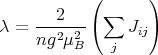
for λ and C:
C∕T for T ≫ TC, but as we approach
TC from above, the susceptibility diverges. This indicates that at the transition
temperature (T = TC), the system can acquire a spontaneous magnetization even in the
absence of an external field, i.e., it becomes ferromagnetic. If we plug in our expressions
for λ and C:
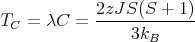 | (22) |
where TC is the Curie temperature. This is reasonable since the energy of a given spin S in the field of its neighbors is ~ zJS2. Notice that T C is proportional to the exhange energy J and to the number of neighbors z.
 | (23) |
and has eigenvalues
 | (24) |
The partition function is
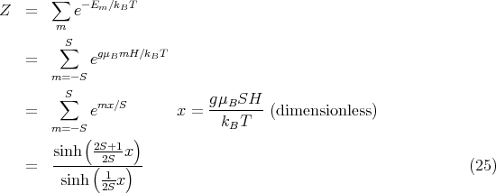
![[ (2S+1 )]
sinh 2S x](lecture1729x.png) - ln
- ln ![[ ( x-)]
sinh 2S](lecture1730x.png) , we get
, we get
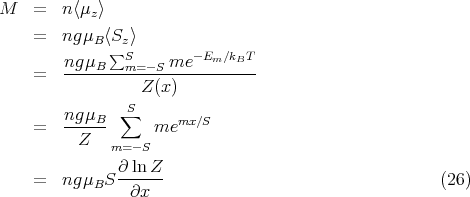
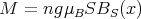 | (27) |
where the Brillouin function
 | (28) |
For S = 1∕2,
 | (29) |
If we define a dimensionless field h = gμBH∕kBT, then
 | (30) |
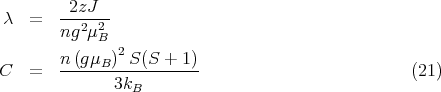
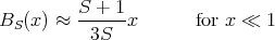
Aside: Let us take a moment to derive the expression for the Curie constant C in Eq. (21). At high temperatures or small fields, hS ≪ 1. For x ≪ 1
 | (31) |
Plugging this into Eq. (30) yields
 | (32) |
Plugging in h = gμBH∕kBT gives
 | (34) |
This is where Eq. (21) came from.
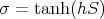
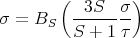
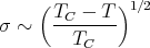
Now back to mean field theory. Eq. (30) is a self-consistent equation for M because H = Hext + λM. To solve for M, some numerical or graphical method of solution must be employed. The graphical procedure of Weiss is probably the simplest method. To use this, rewrite the equation for M in terms of a reduced magnetization σ:
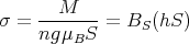 | (35) |
For S = 1∕2,
 | (36) |
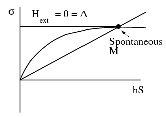
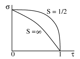
This gives one curve. The other curve comes from
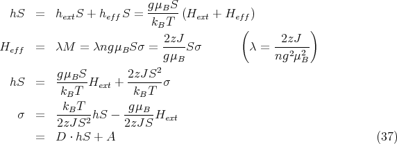
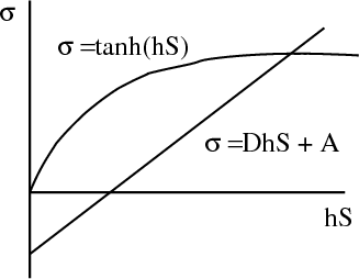
The most important result of the Weiss theory is that when Hext = 0 and the straight line passes through the origin, there is still a non-zero solution for σ, i.e., a spontaneous magnetization is predicted. The general behavior of the spontaneous magnetization can be inferred without extensive calculations. The slope of the straight line is proportional to T (D ∝ T), and rotating the line about the origin corresponds to changing the temperature. When T → 0, σ → 1, and the material becomes completely magnetized. As T is increased, the spontaneous magnetization is reduced and finally vanishes when the slope of the line is equal to the initial slope of the Brillouin function. This occurs at the Curie temperature TC that we found earlier.
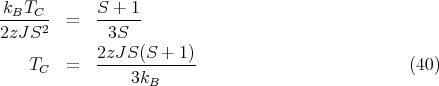
We can solve for TC by matching the slopes at x = 0 of the Brillouin function and the straight line:
 | (38) |
The straight line at small x is given by
 | (39) |
Matching the slopes at T = TC yields
 | (41) |
Solving for hS yields
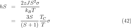
 | (43) |
where τ = T∕TC.
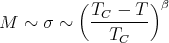
Temperature dependence of the magnetization:
T ~ 0 Mean field theory predicts
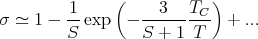 | (44) |
Experiment is closer to spin wave theory:
 | (45) |
For T ~ TC-
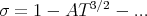
 | (46) |
from mean field theory. In general one writes
 | (47) |
where β is a critical exponent. Experiment finds β ~ 1∕3.
 | (48) |
where r12 = |r1 - r2|, and 1 and 2 are the Hamiltonians of electron 1 and electron 2,
respectively. The electrons are either in a singlet state or a triplet state:
![ψS = √1--[ϕi(1)ϕj(2) + ϕi(2)ϕj(1)]χo
2
-1--
ψT = √ --[ϕi(1)ϕj(2) - ϕi(2)ϕj(1)]χ1 (49)
2](lecture1756x.png)
![χ = √1--[↑↓ - ↓↑]
o 2](lecture1757x.png) | (50) |
and the triplet spin wavefunction (S = 1) is
![(
|{ ↑↑ Sz = 1
χ1 = 1√-[↑↓ + ↓↑] Sz = 0
|( ↓2↓ S = - 1
z](lecture1758x.png) | (51) |
Without the Coulomb interaction, the singlet and triplet are degenerate (have equal energy):
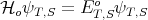 | (52) |
where ET o = E So = E i + Ej. If we include the Coulomb interaction e2∕r 12 using first order perturbation theory, then
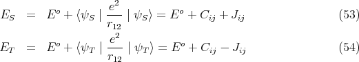
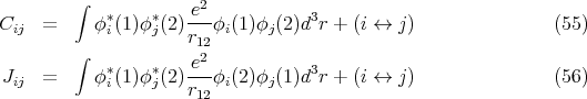
 , and Jij can be either positive or
negative.
, and Jij can be either positive or
negative.
The exchange energy can be rewritten in terms of a spin exchange operator
 | (57) |
which has the property
 | (58) |
where χSms is the spin wavefunction of 2 particles with spin coordinates τ1 and τ2. To
prove this, note that for S = S1 + S2
is the spin wavefunction of 2 particles with spin coordinates τ1 and τ2. To
prove this, note that for S = S1 + S2
![S2 = S21 + S22 + 2S1 ⋅ S2 (59)
1 [ ]
S1 ⋅ S2 = -- S2 - S21 - S22 (60)
2](lecture1766x.png)
 ∕2 and S1 = S2 = 1∕2, S12 = S
1
∕2 and S1 = S2 = 1∕2, S12 = S
1 = 3∕4. So
 ![[ ]
1- 1- 3-
4⃗σ1 ⋅⃗σ2 = 2 S(S + 1) - 2
[ ] {
⃗σ1 ⋅⃗σ2 = 2 S (S + 1) - 3- = - 3 for S = 0 (61)
2 1 for S = 1](lecture1769x.png)
![σ ms 1 ms
P χS=1 (τ1,τ2) = 2-[1 + ⃗σ1 ⋅⃗σ2 ]χS=1 (τ1,τ2)
ms
= χ 1 (τ1,τ2)
= χms1 (τ2,τ1) (62)](lecture1770x.png)
![σ ms=0 1 ms=0
P χS=0 (τ1,τ2) = 2-[1 - 3]χS=0 (τ1,τ2)
0
= - χ0(τ1,τ2)
= χ00 (τ2,τ1) (63)](lecture1771x.png)
 | (64) |
Thus we can write
![o m σ m
E = E + Cij - Jij⟨χ Ss | P | χSs⟩
o [1 ]
= E + Cij - Jij --(1 + ⟨⃗σ1 ⋅⃗σ2⟩)
{ 2
= ES if S = 0 (65)
ET if S = 1](lecture1773x.png)
 | (66) |
We now make a rather bold leap of faith and assume that we can write a similar Hamiltonian for a system with many electrons.
 | (67) |
This is the Heisenberg Hamiltonian and Jij are called the exchange constants. Usually one writes
 | (68) |
where the factor of 4 is from (S = σ∕2)2.