For example, at low temperatures thermodynamic properties are dominated by the low energy excited states. So we do not need to find all the energy eigenstates; we just need to describe these low energy states accurately. If the system is ordered at low temperatures, these low-lying excited states are “collective modes.” For example, in a crystal the atoms are located on lattice sites. The collective modes are normal modes of vibration, i.e., sound waves. Quantized sound waves are called phonons which are analogous to photons. Another example is a ferromagnet where all the spins are lined up parallel to each other in the ground state. The low energy excited states correspond to spin waves which are called magnons when quantized.

We can also sometimes solve interacting systems in the high temperature limit where kT is large compared to the mean energy of interaction. In the infinite temperature limit the interactions are negligible. At high temperatures the interactions can be treated as a perturbation and one can do things like high temperature series expansions.

We will now consider some examples of interacting systems.

(1)

The kinetic energy of the solid is given by

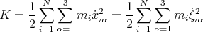(2)

where ẋ_iα = _iα is the αth component of the velocity of the ith atom.

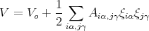
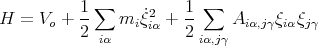
Since the displacements are small, we can expand the potential energy V = V (r₁,...,r_N) in a Taylor series:

(3)

where i and j go from 1 to N; and α and γ go from 1 to 3. The derivatives are evaluated at the equilibrium positions r_i^(o) of the atoms. The first term V _o is the potential energy when the atoms are in their equilibrium configuration. Since this is a minimum of V , the first derivative must vanish: _o = 0, i.e., there is no force on any atom in the equilibrium configuration. So the first term in the Taylor series vanishes. For the second term, let

(4)

We can neglect higher order terms since the displacements ξ are small. So we obtain

(5)

and the Hamiltonian becomes

(6)

The kinetic energy is simple since it is just a sum of terms, each of which just involves one coordinate. But the potential energy is complicated since it involves cross terms coming from different atoms and different coordinates. This is the result of interactions. Since the potential energy is quadratic in the coordinates, we can eliminate this complication by finding the normal modes of the solid. This amounts to making a linear transformation to a new set of normal coordinates q_s:

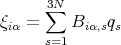(7)

such that a proper choice of coefficients B_iα,s transforms the Hamiltonian to the simple (diagonal) form:

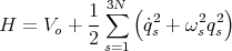(8)

Now we have a sum over independent harmonic oscillators with no cross terms. Each oscillator has frequency ω_s, and its quantum mechanical energy is given by

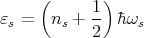(9)

where n_s = 0, 1, 2 ... The total energy is the sum of these one dimensional harmonic oscillator energies:

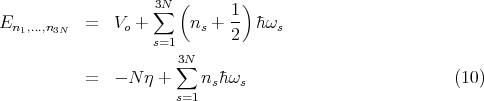
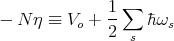(11)

is a constant independent of n_s. ℏω_s∕2 is the zero point energy. η represents the binding energy per atom in the solid at absolute zero.

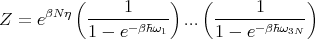
It is now straightforward to calculate the partition function which follows what we did for the Einstein oscillators (see calculation of the Einstein specific heat in lecture 11).

(13)

So we have

(14)

Now we take the logarithm to get ln Z:

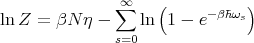(15)

We can convert this sum into an integral by defining σ(ω)dω to be the number of normal modes with angular frequencies in the range between ω and ω + dω.

(16)

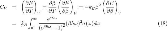
The mean energy of the solid is

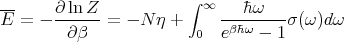(17)

The heat capacity at constant volume is

(19)

If the temperature is high enough such that βℏω_max ≪ 1, then βℏω ≪ 1 for all relevant ω, and we can expand the exponential:

(20)

Then for kT ≫ℏω_max,

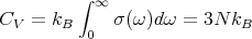(21)

since the integral over σ(ω) is simply the total number of modes:

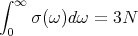(22)

Eq. (21) is the Dulong-Petit law that we obtained earlier by applying the equipartition theorem.

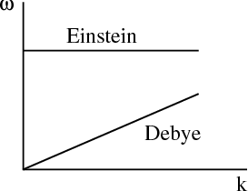
For an elastic continuum, the dispersion relation is ω = c_sk where c_s is the speed of sound. This has the same form as the dispersion relation for photons. From our previous derivation for the density of states in lecture 14, we can write

(23)

where the factor of 3 accounts for the 3 phonon polarizations: 1 longitudinal mode and 2 modes transverse to the direction of propagation with wavevector k.

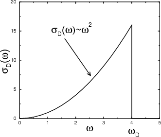
The Debye approximation approximates σ(ω) with σ_D(ω) defined by

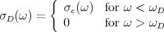(24)

where the “Debye frequency” ω_D is chosen so that σ_D(ω) yields the correct total number of 3N normal modes:

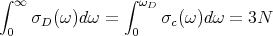(25)

This normalization determines ω_D:

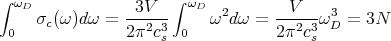(26)

Solving for ω_D yields

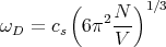(27)

For typical numbers: c_s ≈ 5 × 10⁵ cm/sec, a ≈ (V∕N)^1∕3 ≈ 1Å, ω _D ≈ 10¹⁴ sec^-1 ≈ 100 THz. The corresponding wavelength 2πc_s∕ω_D ~ a. The corresponding Debye temperature Θ_D is defined by kΘ_D ≡ℏω_D. Typically the Debye temperature is of order 300 K.

Notice that the Debye density of states is quadratic in ω.

Using the Debye approximation, the heat capacity becomes

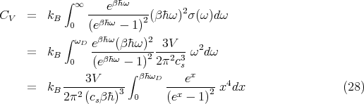
(29)

we can write

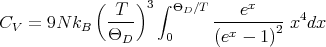(30)

As we have seen, at high temperatures, this reduces to the Dulong-Petit law. At low temperatures, T ≪ Θ_D and we can replace the upper limit of the integral with ∞ and the integral becomes a constant. As a result, we can see immediately that

(31)

More precisely, the integral can be evaluated exactly:

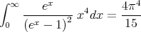(32)

This yields

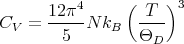(33)

Notice that C_V ~ T³ at low temperatures (T ≪ Θ _D). This provides a reasonably good fit at low temperatures, though it may be necessary to go to temperatures as low as T < 0.02Θ_D. The Debye specific heat certainly gives better agreement with experiment at low temperature than the exponential temperature dependence predicted by the Einstein specific heat (see lecture 11). The Einstein specific heat makes the approximation that all the oscillators have a single frequency ω_E:

(34)

Plugging this into Eq. (18) and using ℏω_E = k_BΘ_E yields our previous result for the Einstein heat capacity from lecture 11:

(35)

Figure 10.2.2 in Reif shows a comparison of the Debye and Einstein specific heats. Both have an S-shape:

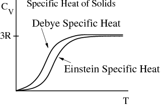
The Debye approximation is good for the acoustic phonon modes while the Einstein approximation is good for the high energy optical phonon modes.