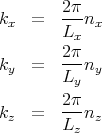
We will focus on the conduction electrons. For simplicity we can describe them as free electrons which means that we neglect their Coulomb interactions. So we can regard the electrons as a gas but because their density is high, their de Broglie wavelength is much larger than their mean separation (see Reif 7.4). This means that the classical approximation breaks down and we have to use quantum statistics. The first thing to understand is that the electrons fill a Fermi sea. To understand this, recall the eigenstates for a particle in a box with periodic boundary conditions. We found that the momentum acquires discrete values
 = ℏ
= ℏ and the numbers nx, ny, and nz are any set of integers– positive,
negative, or zero. We can imagine setting up coordinate axes kx, ky, and kz and putting a point
everywhere in k-space that there is an allowed state. Notice that as the size of the box gets
bigger, the states get closer together in k-space. Since E = ℏ2k2∕2m, the lower energy
states are the ones which are closer to the origin in k-space. Now let’s put in our
conduction electrons. We will fill the states in order of increasing energy. Only 2 electrons
(spin up and spin down) can go into each state. After we’ve finished putting all our
electrons into the states in k-space, we have what is called a Fermi sea. In our case the
Fermi sea will be a sphere in k-space. The surface of this sphere is called the Fermi
surface. The Fermi energy EF is the energy of a state at the Fermi surface, and the
Fermi wavevector kF is the radius of the Fermi sea. So in our case EF = ℏ2k
F 2∕2m.
An electron buried in the depths of the Fermi sea can’t really jump to a nearby
state in k-space because the nearby states are occupied. So these electrons don’t
contribute to the electric current. It’s the electrons near the Fermi surface that can make
transitions to unoccupied states above the Fermi surface and contribute to the electrical
conduction. How near to the Fermi surface do the electrons have to be? Within kBT of
EF .
and the numbers nx, ny, and nz are any set of integers– positive,
negative, or zero. We can imagine setting up coordinate axes kx, ky, and kz and putting a point
everywhere in k-space that there is an allowed state. Notice that as the size of the box gets
bigger, the states get closer together in k-space. Since E = ℏ2k2∕2m, the lower energy
states are the ones which are closer to the origin in k-space. Now let’s put in our
conduction electrons. We will fill the states in order of increasing energy. Only 2 electrons
(spin up and spin down) can go into each state. After we’ve finished putting all our
electrons into the states in k-space, we have what is called a Fermi sea. In our case the
Fermi sea will be a sphere in k-space. The surface of this sphere is called the Fermi
surface. The Fermi energy EF is the energy of a state at the Fermi surface, and the
Fermi wavevector kF is the radius of the Fermi sea. So in our case EF = ℏ2k
F 2∕2m.
An electron buried in the depths of the Fermi sea can’t really jump to a nearby
state in k-space because the nearby states are occupied. So these electrons don’t
contribute to the electric current. It’s the electrons near the Fermi surface that can make
transitions to unoccupied states above the Fermi surface and contribute to the electrical
conduction. How near to the Fermi surface do the electrons have to be? Within kBT of
EF .
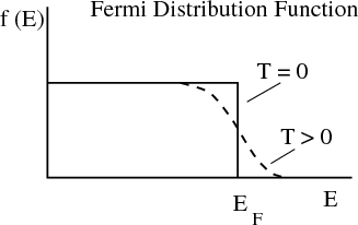
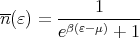
This picture is consistent with the Fermi distribution.
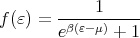 | (1) |
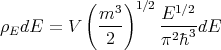
At T = 0 the Fermi distribution is a step function that tells us that the states below the Fermi energy are occupied and those above are unoccupied. The chemical potential at T = 0 is called the Fermi energy, EF = μ(T = 0). The Fermi energy depends on how many electrons there are; the more electrons, the larger the Fermi energy. More precisely, the higher the density of electrons, the higher the Fermi energy. We can calculate this dependence as follows. Since all states with k ≤ kF are occupied at T = 0, we have
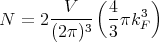 | (2) |
where the factor of 2 is for the 2 possible spin states of an electron. Or
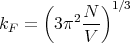 | (3) |
or
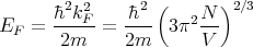 | (4) |
We can define a characteristic temperature which is called the Fermi temperature
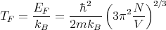 | (5) |
Typically the Fermi temperature is on the order of kBT ~ 1 eV ~ 10,000 K. So room temperature (300 K) is much less than TF . At room temperature the electrons behave a lot like they do at zero temperature. When we say low temperature for electrons, we mean T ≪ TF . In this case the Fermi distribution is a little smeared but still looks step-like. We speak of a “degenerate” Fermi gas. By degenerate, we mean there are a lot of electrons with the same energy, namely the Fermi energy. If T ≫ TF , then we are in the classical, nondegenerate limit.
A good example of a degenerate Fermi gas are the electrons in a metal. At first glance, it would appear that the noninteracting approximation would be totally inappropriate because of the obvious Coulomb interactions among the electrons. Two comments should be made. (1) More sophisticated theory indicates that a noninteracting, single particle approximation is valid but the particles are not true electrons but rather “quasiparticles” with energy ε = ℏ2k2∕2m* where m* is an “effective mass.” This approximation improves as the temperature is lowered. (2) We can compute the consequences of the simple non–interacting assumption and compare the results to experimental data. The agreement is excellent.
Consider a typical metal like Copper (Cu). If one plugs the appropriate numbers into (5),
then one finds that TF  80, 000 Kelvin (see page 391 of Reif). This is well above the melting
point of copper, so for any temperature below the melting point, we can use the low
temperature approximation.
80, 000 Kelvin (see page 391 of Reif). This is well above the melting
point of copper, so for any temperature below the melting point, we can use the low
temperature approximation.
One of the many quantities of interest is the contribution of the electrons in a metal to the
total specific heat of the solid. (The other big contributor are the lattice vibrations or
phonons.) Classically, using the equipartition theorem, we expect the electrons to contribute
 R to the molar specific heat. Yet at room temperature, the observed specific heat of both
metals and insulators is 3R. This is the classical Dulong-Petit result that we got by just
considering vibrations of the atoms and ignoring the electrons. So it appears that the electrons
don’t contribute to the specific heat at room temperature. In other words, they aren’t behaving
classically.
R to the molar specific heat. Yet at room temperature, the observed specific heat of both
metals and insulators is 3R. This is the classical Dulong-Petit result that we got by just
considering vibrations of the atoms and ignoring the electrons. So it appears that the electrons
don’t contribute to the specific heat at room temperature. In other words, they aren’t behaving
classically.
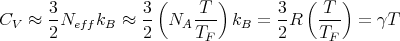
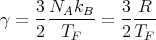
Because of the Pauli principle, only those electrons within a few kBT of the Fermi energy are capable of being excited into higher energy levels and changing their state. Most of the electrons are far below the Fermi energy, cannot change their state because all the states near them in energy are occupied, and therefore do not participate in thermal processes. We can assume that only a fraction of the electrons can contribute to the specific heat. This fraction ~ T∕TF ≪ 1. Thus we can approximate the molar specific heat by
 | (6) |
where
 | (7) |
This says that the low temperature specific heat of metals should contain a term proportional to T. This is indeed observed.
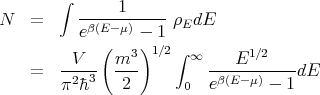
Reif does a proper calculation of the specific heat CV for a free electron gas in section 9.17. One starts with the mean energy
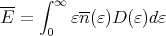 | (8) |
where D(ε) is the number of states lying between ε and ε + dε. The thermal occupation factor is the Fermi function:
 | (9) |
The specific heat is just the derivative of E:
 | (10) |
We won’t go through the calculation (see Reif 9.17). The answer for the molar specific heat is
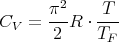 | (11) |
The fact that electrons have both spin–up and spin–down states is included in here. Note that the specific heat is linear in T.
Interesting things happen at very low temperatures and Bose–Einstein condensation is one of them. Recall that there is no statistical limit to the number bosons that can occupy a single state. In a Bose condensed state, an appreciable fraction of the particles is in the lowest energy level at temperatures below TC. These particles are in the same state and can be described by the same wavefunction. In other words a macroscopic number of particles are in one coherent state. If we write ψ = |ψ|eiϕ, then this state is described by a given phase ϕ.
The oldest known physical manifestation of Bose condensation is superfluid 4He. A 4He atom has total angular momentum zero and is therefore a boson. At TC = 2.18 K liquid helium becomes superfluid. The transition temperature is called the λ-point because the shape of the specific heat curve at TC is shaped like λ. One cools liquid helium by pumping on it to get rid of the hot atoms (evaporative cooling). It boils a little. Then at the transition it boils vigorously and suddenly stops. The reason for this behavior is that the thermal conductivity increases by a factor of about 106 at the transition, so that the superfluid is no longer able to sustain a temperature gradient. To make a bubble, heat has to locally vaporize the fluid and make it much hotter than the surrounding fluid. This is no longer possible in the superfluid state.
Perhaps the hallmark of a superfluid is that it has no viscosity. As a result the superfluid can flow through tiny capillary tubes that normal liquid can’t get through. Superfluid 4He is often described by a two–fluid model, i.e., it is thought of as consisting of 2 fluids, one of which is normal and the other is superfluid. It’s the superfluid component which is able to flow through the capillary tube. So if you use this method to measure the coefficient of viscosity, you find that it suddenly drops to zero at the λ-point.
One can see the effect of both components by putting a torsional oscillator consisting of a stack thin, light, closely spaced mica disks immersed in the liquid. If the liquid has a high viscosity, the liquid between the disks is dragged along and contributes significantly to the moment of inertia of the disks. If the viscosity is small, the moment of inertia is more nearly equal to that of the disks alone. Using this method, no discontinuity is found in the coefficient of viscosity at the λ-point.
Another weird thing that superfluid helium does is escape from a beaker by crawling up the sides, flowing down the outside, and dripping off the bottom. The helium atoms are attracted by the van der Waals forces of the walls of the container, and they are able to flow up the walls because of the lack of viscosity. The rate of flow can be 30 cm per second or more. The superfluid helium can surmount quite a high wall, on the order of several meters in height.
(Brief aside to explain the van der Waals force: As an electron moves in a molecule, there exists at any instant of time a separation of positive and negative charge in the molecule. The latter has, therefore, an electric dipole moment p1 which varies in time. If another molecule exists nearby, it will have a dipole moment induced by the first molecule. These two dipoles are attracted to each other. This is the van der Waals force.)
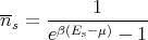
We can show mathematically that there is a macrosopic population of the lowest energy state in the following way. Consider a gas of noninteracting bosons. Let the energy levels be measured from the lowest energy level, i.e., let the zero point energy be the zero of energy. Then the chemical potential μ must be negative, otherwise the Bose–Einstein distribution would be negative for some of the levels. Recall from lecture 13 that the Bose–Einstein distribution gives the average number of particles in state s:
 | (12) |
μ is adjusted so that the total number of particles is N:
 | (13) |
Let me give a sneak preview: If we assume a continuous distribution of states, μ starts out negative and gets bigger as the temperature decreases. μ equals its upper limit of zero at some temperature TC, below which we can no longer satisfy (13) because the right hand side can’t deliver enough particles. This leads us to treat the lowest energy level separately and we find that we can satisfy (13) by keeping the extra particles we need in the lowest state.
Now let’s do the math. In order to turn the sum over s in (13) into an integral, let’s assume a continuous density of states. In lecture 14 we found that if k–space is isotropic, i.e., the same in every direction, then the number of states in a spherical shell lying between radii k and k + dk is
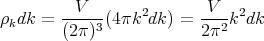 | (14) |
Now if the energy of the bosons is purely kinetic energy and continuous, then
 | (15) |
and
 | (16) |
or
 | (17) |
Also (15) implies that
 | (18) |
Plugging (17) and (18) into (14) yields
 | (19) |
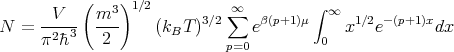
So we can rewrite (13) as
Now recall that for a geometric series
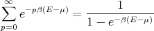 | (20) |
So
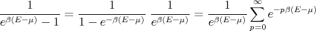 | (21) |
Plugging this into (20) leads to
 | (22) |
Let x = βE. Then
 | (23) |
Let s = p + 1 and y = sx. Then
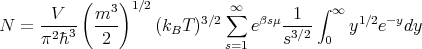 | (24) |
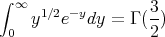
The definition of a gamma function is
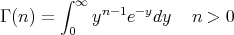 | (25) |
(Aside: Γ(n) = (n - 1)! if n is a positive integer.) So
 | (26) |
Thus
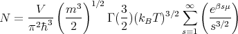 | (27) |
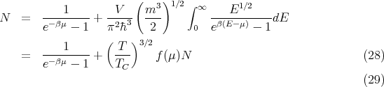
Now on the right hand side, as the temperature T decreases, μ must increase to keep the product constant and equal to N. T can be made as small as we wish, but μ, which we said must be negative, cannot be greater than zero. But the product must be a constant. So (27) is only valid above a certain critical temperature TC. Below this temperature, our treatment breaks down. Where did we go wrong? The flaw lies in the fact that we assumed that the states are continuously distributed. However, since we are interested in very low temperatures which involves the occupation of the lowest lying energy levels, we may expect that the actual discrete nature of the level distribution might play an essential role in the lowest temperature range. So let us treat the lowest level E1 = 0 separately. We will assume that it is not degenerate with any other levels and we will assume that the remaining levels are continuously distributed from E = 0 to E = ∞ as described by (19). So in our summation (13) we will treat the lowest level separately:
where the second quantity on the right is just the right hand side of (27), written in terms of the critical temperature TC. f(μ = 0) = 1 because TC is defined such that the right hand side of (27) equals N with T = TC and μ = 0.We see that it is now possible to satisfy this new equation with negative values of μ for all temperatures, since the first term becomes infinite as μ → 0. The inclusion of the lowest energy level as a separate term in our treatment has thus removed the previous difficulty of not being able to account for all of the particles at temparatures below TC. If we now inquire into what this equation means physically, we see that, at temperatures below TC, the chemical potential μ will take on such values that those particles which are not included in the continuous distribution will be found in the lowest level. That is, a kind of condensation occurs; it is such that an appreciable fraction of the particles is in the lowest energy level at temperatures below TC.
If we write (29) as
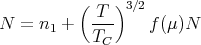 | (30) |
and realize that f(μ ≈ 0) ≈ 1 at low temperatures, then we find the population n1 of the lowest level to be, approximately,
![[ ( T )3∕2]
n1 = N 1 - ---
TC](lecture1536x.png) | (31) |
At T = TC, n1 = 0 while at T = 0, n1 = N. Using n1 = (e-βμ - 1)-1, we find that at low temperatures
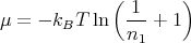 | (32) |
Notice that μ is negative. As T → 0, μ → 0:
 | (33) |
Considering superfluid helium as a 2 component fluid with normal and superfluid components is consistent with having some of the particles in the lowest energy level and the rest in higher energy levels. There is no microscopic theory of superfluid helium, though computer simulations by Ceperley have been quite successful in reproducing its properties. One of the complications is that the helium atoms are so closely packed that they are strongly interacting; they’re in a liquid state. It would be closer to the ideal case to have a system of bosons which are weakly interacting.
(Reference: H.–J. Miesner and W. Ketterle, “Bose–Einstein Condensation in
Dilute Atomic Gases,” Solid State Communications 107, 629 (1998) and references
therein.)
This has recently been achieved in the case of alkali atoms such as rubidium, sodium, and
lithium. Using a combination of optical and magnetic traps together with laser cooling and
evaporative cooling, several research groups have achieved Bose condensation in dilute weakly
interacting vapors of alkali atoms. In these systems the thermal deBroglie wavelength exceeds
the mean distance between atoms. Nanokelvin temperatures and densities of 1015 cm-3 have
been achieved. (Compare this to a mole of liquid which has a typical density of 1023 cm-3.)
At nanokelvin temperatures the thermal deBroglie wavelength exceeds 1 μm which
is about 10 times the average spacing between atoms. In these experiments they
have actually been able to directly observe the macroscopic population of the zero
momentum eigenstate. In addition the coherence resulting from being in macroscopic
wavefunctions has been demonstrated by observing the interference between two independent
condensates. Two spatially separated condensates were released from the magnetic trap and
allowed to overlap during ballistic expansion of the gases. Interference patterns were
observed that are analogous to the pattern produced in a double–slit experiment in
optics.