|
| (1) |
have quantized energy levels. For example, a particle of mass m in a box with infinitely high walls, has energy levels given by
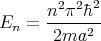 | (2) |
where n = 1, 2, 3,.... A harmonic oscillator is another example. The energy eigenvalues are
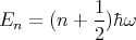 | (3) |
where n = 0, 1, 2, 3,.... Notice once again that the energy levels are quantized. In this case they are evenly spaced by an amount ΔE = ℏω.
Electromagnetic radiation is also quantized. Light can be described as waves or as
particles called photons. A photon has energy hν where ν is the frequency of the
electromagnetic wave. Recall that ω = 2πν and that ν = c∕λ where c is the speed
of light. Often one speaks in terms of the wavenumber k = 2π∕λ. If we make it a
vector quantity  , then we call it a wavevector. This is related to the momentum by
 = ℏ
= ℏ and to the frequency by ω = ck. So if the electromagnetic wave has a short
wavelength, it has a high frequency and the photon carries a lot of energy. Lots of
wiggles means lots of energy. Photons are massless and they travel at the speed of
light.
and to the frequency by ω = ck. So if the electromagnetic wave has a short
wavelength, it has a high frequency and the photon carries a lot of energy. Lots of
wiggles means lots of energy. Photons are massless and they travel at the speed of
light.
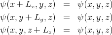
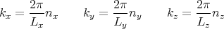
Suppose we have a 3 dimensional box whose walls are parallel to the x, y, and z axes with lengths Lx, Ly, and Lz. Thus the volume is V = LxLyLz. We can solve this as a particle in a box problem. Inside the box the potential is zero. The eigenmodes are waves. However, let’s choose boundary conditions such that the solution of Schroedinger’s equation are wavefunctions that are plane waves:
![Ψ = A exp [i(⃗k ⋅⃗r - ωt)] = ψ(⃗r)exp (- iωt)](lecture146x.png) | (4) |
This is a propagating wave that is never reflected. So our box can’t have hard walls. Rather let’s imagine that our box is embedded in an infinite set of similar boxes in each of which the physical situation is exactly the same. In other words, each of these boxes is a repeat of the original box.

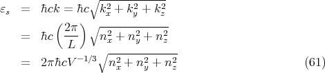
To describe this situation, we use periodic boundary conditions which we can write as
![ψ (⃗r) = exp(i⃗k ⋅⃗r) = exp[i(kxx + kyy + kzz)]](lecture149x.png) | (5) |
to satisfy these boundary conditions, then we must require that
 | (6) |
where nx is an integer. We can rewrite this as
 | (7) |
Similarly,
We can use p = ℏk and E = p2∕2m to deduce that
 | (8) |
Once again we see that the energy levels are quantized. Notice that for any kind of macroscopic volume where Lx, Ly, and Lz are large, the energy levels are very closely spaced.
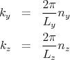
Now we want to count the number of modes or waves that have wavevectors between
 = (kx,ky,kz) and
  + d
+ d = (kx + dkx,ky + dky,kz + dkz). For given values of ky and kz, it
follows from (7) that the number Δnx of possible integers nx for which kx lies in the range
between kx and kx + dkx is equal to
= (kx + dkx,ky + dky,kz + dkz). For given values of ky and kz, it
follows from (7) that the number Δnx of possible integers nx for which kx lies in the range
between kx and kx + dkx is equal to
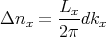 | (9) |
We see that if Lx is very large, a lot of states can be in the small interval dkx. The same
holds true for dky and dkz. So the number of states that lie between  and
and  + d
+ d is
is
 | (10) |
or
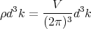 | (11) |
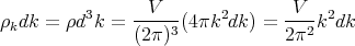
where d3k ≡ dk
xdkydkz is an element of volume in “k space.” Notice that the number of states
ρ is independent of  and proportional to the volume V under consideration. So the “density of
states”, i.e., the number of states per unit volume, lying between
and proportional to the volume V under consideration. So the “density of
states”, i.e., the number of states per unit volume, lying between  and
and  + d
+ d is d3k∕(2π)3
which is a constant independent of the magnitude or shape of the volume V . Note that ρ
denotes the number of single particle states.
is d3k∕(2π)3
which is a constant independent of the magnitude or shape of the volume V . Note that ρ
denotes the number of single particle states.
Using the relation  = ℏ
= ℏ , we can also deduce that the number of states ρpd3p in the
momentum range between
, we can also deduce that the number of states ρpd3p in the
momentum range between  and
and  + d
+ d is
is
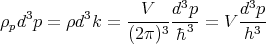 | (12) |
where h = 2πℏ is the ordinary Planck’s constant. Notice that V d3p is the volume of the
classical 6 dimensional phase space occupied by a particle in a box of volume V and with
momentum between  and
and  + d
+ d . Thus (12) shows that subdivision of this phase space into
cells of size h3 yields the correct number of quantum states for the particle. If we compare this
to our classical expression V d3p∕h
o3, we see that our arbitrary length h
o is replaced by Planck’s
constant h.
. Thus (12) shows that subdivision of this phase space into
cells of size h3 yields the correct number of quantum states for the particle. If we compare this
to our classical expression V d3p∕h
o3, we see that our arbitrary length h
o is replaced by Planck’s
constant h.
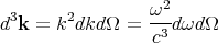
If k–space is isotropic, i.e., the same in every direction, then the number of states in a spherical shell lying between radii k and k + dk is
 | (13) |
If we are considering photons for which ω = ck, then we can plug k = ω∕c into (13) to get the number of states lying between ω and ω + dω.
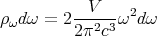 | (14) |
The factor of 2 comes from the fact that there are 2 photon polarizations. The polarization
refers to the direction of the electric field vector  in the electromagnetic radiation. Since
  must be perpendicular to
  , there are 2 polarization directions. We will use (14) in deriving
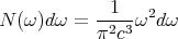
blackbody radiation. Sometimes the term “density of states” for photons is used to refer to the
number of states per unit volume per unit energy:
, there are 2 polarization directions. We will use (14) in deriving
blackbody radiation. Sometimes the term “density of states” for photons is used to refer to the
number of states per unit volume per unit energy:
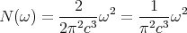 | (15) |
The density of states is very useful for converting sums into integrals as we shall see.
 | (16) |
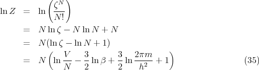
where the partition function Z
 | (17) |
This is for the canonical ensemble with fixed temperature T and fixed particle number N. We have seen that ln Z is very useful in finding other quantities. For example,
 | (18) |
 | (19) |
 | (20) |
 | (21) |
 | (22) |
But the problem is that it is very difficult to solve Schroedinger’s equation to get ER:
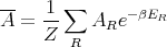
 | (23) |
It is much easier to solve Schroedinger’s equation to get single particle energies. So we consider systems (gases) of noninteracting particles. If we know how many particles are in each single particle state, then we just sum over all the particles to get the appropriate average, e.g., the mean energy of the whole system. If we have to treat the particles quantum mechanically because their wavefunctions overlap or because the temperature is low, then we need to pay attention to whether the particles are fermions or bosons. Fermions can have at most one particle in a state while bosons can have umpteen particles in a state. So now the mean energy is given by
 | (24) |
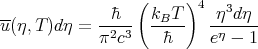
where the mean number of particles in state s is given by
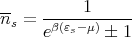 | (25) |
+ is for fermions and - is for bosons. It’s usually not easy to do sums, so it would be nice if we could convert the sum into an integral. That’s why we calculated density of single particle states. Then we can do the conversion:
 | (26) |
or
 | (27) |
So the mean energy becomes
 | (28) |
where
 | (29) |
 | (30) |
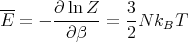
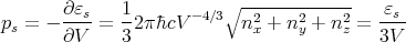
where ζ is the partition function for one particle.
![∑
ζ = e-βεr
r [ ]
∑ βh¯2 ( 2 2 2)
= exp - ---- k x + k y + kz (31)
kx,ky,kz 2m](lecture1457x.png)
 | (32) |
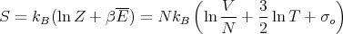
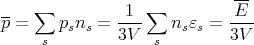
Since the number of allowed k states is very large and since these states are very close together with spacing going as 1∕L, we can approximate the sum by an integral. This is where the density of states comes in handy.
 | (33) |
So
![∫ ∞ [ 2 2]
ζ = -V-- exp - β¯h-k-- k2dk
2π2 0 2m
√ --( )3∕2
= -V----π- -2m-
2π2 4 β ¯h2
V
= -3-(2πmkBT )3∕2 (34)
h](lecture1460x.png)
 | (36) |
and
 | (37) |
where
 | (38) |
This is identical to the result obtained for the purely classical ideal gas except that σo now has a well defined value with ho = h = Planck’s constant and the Gibbs paradox has automatically been taken care of.
 | (39) |
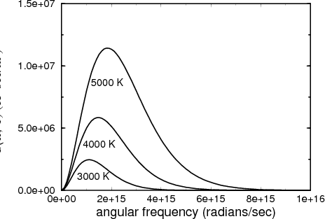
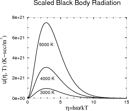
One can imagine making a histogram by counting the photon energy density in each frequency range from ω to ω + dω. It turns out that this distribution of the energy density of blackbody radiation is a universal curve that depends only on the temperature T. In other words if one plots the distribution of the photon energy density (counting both directions of polarization) as a function of photon (angular) frequency ω, the shape of the curve is universal and the position of the peak is a function only of the temperature. When we say that the curve is universal, we mean that it doesn’t depend on the size or shape of the box, or what the walls are made of. All that matters is the temperature.
Blackbody radiation is historically important in physics for two reasons. The first is that the measurement of the spectral distribution in the late 1800’s led Planck to come up with the idea of energy quantization. He couldn’t explain the distribution unless he postulated that E = hν. This marked the birth of quantum mechanics. The second reason that blackbody radiation is important is that 3 K black body radiation pervades the universe and is the remnant of the Big Bang. This radiation is in the microwave region.
Let’s calculate the distribution of the mean energy density of blackbody radiation. Since the size and shape of the box don’t matter, let’s imagine a rectangular box of volume V filled with a gas of photons that are in thermal equilibrium. The box has edges with lengths Lx, Ly, and Lz such that each of these lengths is much larger than the longest wavelength of significance. There are 2 factors that determine the energy density at a given frequency. The first is the average energy in each state s which is given by
 | (40) |
If we set εs = ℏω and ns = n(ℏω), we can rewrite this to give:
 | (41) |
The second factor is the number of states per unit volume whose frequency lies in the range between ω and ω + dω. This is given by (15)
 | (42) |
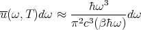
So at temperature T the mean energy density u(ω,T)dω contained in the photon gas by photons whose frequencies are between ω and ω + dω is given by the product of the average energy in each single photon state and the density of states which lie in this frequency range:
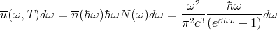 | (43) |
We can rewrite this to give:
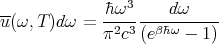 | (44) |
This is Planck’s law for the blackbody spectrum.
We can take the high temperature limit to get the classical limit of this spectrum. In the high temperature limit, β is small so we can expand the exponential in the denominator:
 | (45) |
So the high temperature limit of (44) is
 | (46) |
or, using β = 1∕kBT, we can write
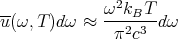 | (47) |
This is the Rayleigh–Jeans formula for blackbody radiation. Notice that eqn. (47) increases as ω2. Therefore the classical spectrum (47) predicts that the energy density goes to infinity as the frequency goes to infinity. By the end of the 1800’s the black body spectrum had been measured and the classical formula had been calculated. There was a clear lack of agreement, so people knew they had a problem. Planck resolved the conflict by proposing that electromagnetic energy was not continuous, but rather was quantized. He proposed E = ℏω (or E = hν) and derived Planck’s law (44). This fit the data very well, and quantum mechanics was born.
We can rewrite (44) in terms of a dimensionless parameter η:
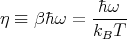 | (48) |
Planck’s law becomes:
 | (49) |
If we plot u(η,T) versus η, the maximum occurs around ηmax ≈ 3.
So if at temperature T1 the maximum occurs at frequency ω1,max, then at some other temperature T2 the maximum occurs at ω2,max. This is because
 | (50) |
or
 | (51) |
This is called the Wien displacement law. It says that
 | (52) |
This was initially an empirical relation that was deduced from the experimental data. We see that it also follows from Planck’s law. It is often useful in physics to express things in terms of dimensionless parameters. The Wien displacement law is an example of useful scaling relations that can result from this.
We can also calculate the total energy density uo(T) contained in the photon gas at temperature T by integrating (44) over frequency:
 | (53) |
Using (49), we can rewrite this as
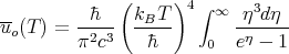 | (54) |
One can evaluate the integral exactly. The answer is
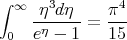 | (55) |
Using this, one finds
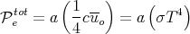
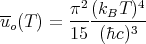
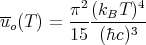 | (56) |
This is known as the Stefan–Boltzmann law. The important point is that the total energy density goes as the fourth power of the temperature:
 | (57) |
Finally the mean pressure p exerted on the walls of the enclosure by the radiation is simply related to the total energy density:
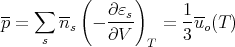 | (58) |
To see where this comes from, recall that
 | (59) |
Now use
 | (60) |
to obtain
 | (62) |
So the average pressure for the system is
 | (63) |
or
 | (64) |
(The pressure can also be written as 
 T = -
T = - T .) The “3” in the denominator
reflects the fact that the box is 3 dimensional. Radiation pressure is quite small, but it is what
gives comets their tails. Solar radiation is what pushes tiny bits of dust and ice that come from
the ice ball away from the sun and produces the tail. The comet tail always points away from
the sun. The power emitted ~ flux ~ cuo(T).
T .) The “3” in the denominator
reflects the fact that the box is 3 dimensional. Radiation pressure is quite small, but it is what
gives comets their tails. Solar radiation is what pushes tiny bits of dust and ice that come from
the ice ball away from the sun and produces the tail. The comet tail always points away from
the sun. The power emitted ~ flux ~ cuo(T).
If this were not true, the body would be losing or gaining energy and would get cooler or would heat up. As a result, its temperature would no longer be the same as the ambient photons at temperature T; it would no longer be in equilibrium. So it must absorb the same amount of power as it emits in order to stay in equilibrium.
We can make an even stronger statement. Namely, that in equilibrium the power radiated and absorbed by the body must be equal for any particular element of area of the body, for any particular direction of polarization, and for any frequency range. To show that this must be true, one could imagine putting a shield or filter around the object that absorbs all radiation except that, in one small element of area, it is completely transparent to radiation in one direction with one polarization and in one narrow frequency range between ω and ω + dω. In the presence of the shield the body must absorb and emit the same power in order to avoid heating up or cooling off, i.e., in order to stay in equilibrium. So the power radiated and absorbed by the body must be equal for any particular element of area of the body, for any particular direction of polarization, and for any frequency range. This is called the principle of detailed balance.
The principle of detailed balance is a fundamental result that is based on very
general arguments. Microscopically it is a result of time reversal invariance and the
fundamental assumption of accessible microstates being equally probable in an isolated
system. Consider a single isolated system consisting of several weakly interacting parts,
e.g., a body and photons. When these parts are not interacting, the system can
be in any one of its quantum states labeled by indices r, s, etc. When interactions
are present, the interactions induce transitions between the states. Let wrs be the
transition rate (or transition probability per unit time) from state r to state s. Under
time reversal, t →-t, r → r* and s → s* where r* and s* are the time reversed
states of r and s. For example, if a particle has momentum  in state r, then it has
momentum -
in state r, then it has
momentum - in state r*. If the system is invariant (the same) under time reversal,
then
in state r*. If the system is invariant (the same) under time reversal,
then
 | (65) |
This expresses the principle of microscopic reversibility. For example, if the body in the cavity
emits a photon with wavevector  , then the time reversed process is the absorption of a photon
with wavevector -
, then the time reversed process is the absorption of a photon
with wavevector - . Microscopic reversibility asserts that these two processes occur with equal
probability.
. Microscopic reversibility asserts that these two processes occur with equal
probability.
If we have some initial set A of states labeled by r and some final set B of states labeled by s, the transition probability from A → B is given by
 | (66) |
where Pr is the probability of being in state r. The probability of landing in state s is the probability Pr of being in state r multiplied by the transition rate wrs to state s. Similarly the time reversed process has a transition rate given by
 | (67) |
But the fundamental postulate of statistical mechanics states that accessible macrostates are equally probable in an isolated system. So Pr = Ps* and
 | (68) |
This is the principle of detailed balance.
 i(k,α) be the
incident radiation power on a unit area of this body per unit frequency and solid angle
range about the vector k with polarization α. Let a(k,α) be the fraction of incident
power absorbed, the rest being reflected. By the principle of detailed balance, the
power absorbed must equal the power emitted e(-k,α) in the opposite direction
-k:
i(k,α) be the
incident radiation power on a unit area of this body per unit frequency and solid angle
range about the vector k with polarization α. Let a(k,α) be the fraction of incident
power absorbed, the rest being reflected. By the principle of detailed balance, the
power absorbed must equal the power emitted e(-k,α) in the opposite direction
-k:
 | (69) |
For a blackbody, a(k,α) = 1; a good absorber is a good emitter and vice-versa. If we integrate
over all directions  and polarizations α, the total power emitted per unit area into the
frequency range between ω and ω + dω is
and polarizations α, the total power emitted per unit area into the
frequency range between ω and ω + dω is
 | (70) |
In the appendix to these notes, we show that
![[ ]
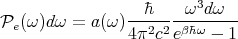
1---
Pe(ω )d ω = a(ω ) 4cu (ω)dω](lecture14107x.png) | (71) |
It makes sense to see cu(ω) for the flux. The factor of 1∕4 comes from geometric considerations. Using Eq. (44), we can write this as
 | (72) |
The total power etot emitted per unit area of the body is obtained by integrating Eq. (72)
over frequency as we did in Eqs. (54)-(56) to obtain
 | (73) |
where uo is given by Eq. (56):
 | (74) |
Eq. (73) is another form of the Stefan-Boltzmann law. The Stefan-Boltzmann constant σ is
 | (75) |
For a perfect blackbody, a = 1. For something shiny like gold, a ≈ 0.01.
Let i(k,α) be the incident radiation power on a unit area of this body per unit frequency
and solid angle range about the vector k with polarization α. Let a(k,α) be the fraction of
incident power absorbed, the rest being reflected. By the principle of detailed balance, the
power absorbed must equal the power emitted e(-k,α) in the opposite direction
-k:
 | (76) |
For a blackbody, a(k,α) = 1; a good absorber is a good emitter and vice-versa.
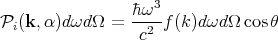
Let us now calculate explicitly the power i(k,α) incident per unit area of a body in an
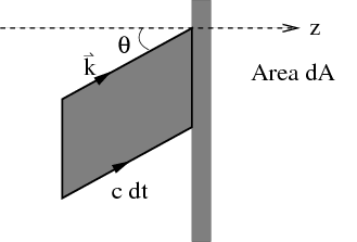
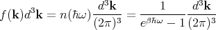
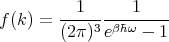
enclosure at temperature T. This is the incident energy flux. Let f(k)d3k be the mean number
of photons per unit volume with a given polarization whose wavevector lies between k
and k + dk. So (c dt cos θ)f(k)d3k photons of a given frequency and polarization
strike a unit area of the body in a time dt. Since each photon carries energy ℏω, one
obtains
 | (77) |
Converting d3k to spherical coordinates and using k = ω∕c, we obtain
 | (78) |
and
 | (79) |
If the body absorbs isotropically, then the fraction of incident radiation absorbed is a(k,α) = a(ω), i.e., a is independent of the direction k. We are also assuming a is independent of the polarization direction. So the power emitted in the direction k′ = -k is
 | (80) |
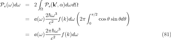
Now let us find the total power e(ω)dω emitted per unit area into the frequency
range between ω and dω for both polarization directions by integrating over the solid
angle. Using dΩ = sin θdθdϕ and multiplying by 2 for both polarizations, we write
 | (82) |
or
 | (83) |
We can relate this to the expression for the mean radiation density (Eq. (44)):
![[ ]
Pe(ω )dω = a(ω ) 1-cu(ω)dω
4](lecture14122x.png) | (85) |
It makes sense to see cu(ω) for the flux. This is Eq. (71) in the lecture notes.