
 ,
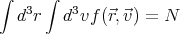
, )d3rd3v be the mean number of molecules with
center of mass position between
)d3rd3v be the mean number of molecules with
center of mass position between  and
and  + d
+ d and velocity between
  and
and  + d
+ d .
Then
.
Then
|
| (1) |
where C is a constant determined by normalization. Here we have used the Boltzmann distribution e-βE with the energy E being the kinetic energy of the system mv2∕2. The contribution to the energy from internal states or degrees of freedom doesn’t affect the velocity; these internal states are summed over (∑ r exp(-βϵr)) and will just contribute to C. The constant C is determined by the condition
 | (2) |
We can evaluate the integrals to obtain C:
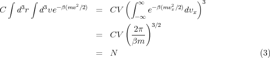
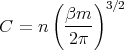 | (4) |
where n ≡ N∕V is the total number of molecules per unit volume. Hence
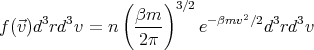 | (5) |
or
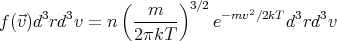 | (6) |
We have omitted  from the argument of f since f doesn’t depend on
  . Equation (6) is known
as the Maxwell velocity distribution for a dilute gas in thermal equilibrium. Notice that it is a
Gaussian distribution centered at v = 0. Recall that the exponential factor in a Gaussian
distribution has the form exp(-x2∕2σ2) where 2σ is the width of the distribution. Then the
width of the Maxwell velocity distribution is σ =
. Equation (6) is known
as the Maxwell velocity distribution for a dilute gas in thermal equilibrium. Notice that it is a
Gaussian distribution centered at v = 0. Recall that the exponential factor in a Gaussian
distribution has the form exp(-x2∕2σ2) where 2σ is the width of the distribution. Then the
width of the Maxwell velocity distribution is σ =  . Notice that the width increases as
the temperature increases. This means there are more hot molecules at higher temperatures.
By “hot” molecules I mean ones with large |v|. This applies for both positive and negative
velocities because in (6) v2 = v
x2 + v
y2 + v
z2 and each component of velocity can be positive or
negative.
. Notice that the width increases as
the temperature increases. This means there are more hot molecules at higher temperatures.
By “hot” molecules I mean ones with large |v|. This applies for both positive and negative
velocities because in (6) v2 = v
x2 + v
y2 + v
z2 and each component of velocity can be positive or
negative.
 | (7) |
where
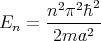 | (8) |
with n = 1, 2, 3,.... n is an example of a quantum number. It’s a number which characterizes an eigenstate of the system. It changes from eigenstate to eigenstate, but if the system is in that eigenstate, it remains in that eigenstate and the quantum numbers describing that state don’t change either. This is why an eigenstate is called a stationary state. Typically the quantum numbers are associated with symmetries. Symmetry means that the system looks the same under certain operations. For example if the system is invariant under time translation, then the Hamiltonian is time independent, and energy is conserved. This was true of the case of a particle in a box, and we labelled the energy eigenstates by n.
Another possible symmetry is spatial translation. If the potential is invariant under spatial
translation, then momentum is a good quantum number. This would be true of a constant
potential or if there were no potential. Classically momentum is conserved as long as the
system is not subjected to a force. So if  = d
= d ∕dt = 0, then
  = constant. The force is the
gradient of the potential:
= constant. The force is the
gradient of the potential:  = -∇V (
 ). So momentum is a good quantum number
as long as the potential does not vary spatially, i.e, as long as it’s constant. (We
don’t usually refer to forces in quantum mechanics.) If the potential is constant
or zero, then we have a free particle with momentum
). So momentum is a good quantum number
as long as the potential does not vary spatially, i.e, as long as it’s constant. (We
don’t usually refer to forces in quantum mechanics.) If the potential is constant
or zero, then we have a free particle with momentum  , energy E = p2∕2m and
ψ ~ exp(i
, energy E = p2∕2m and
ψ ~ exp(i ⋅
⋅ ∕ℏ).
∕ℏ).
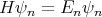
Another way to define a conserved quantity is to recall the Heisenberg equation of motion. For wavefunctions, it takes the form
 | (9) |
There is also an equation of motion for operators. Let  be some operator. Its equation of motion is
![∂Aˆ
i¯h --- = [ ˆA,Hˆ]
∂t](lecture1228x.png) | (10) |
So if iℏ∂Â∕∂t = 0, then we must have [Â,Ĥ] = 0. This is the condition that A is a constant of the motion and is a conserved quantity. So if momentum is a conserved quantity, then it commutes with the Hamiltonian:
![[ ˆH, ˆp] = Hˆ ˆp - pˆˆH = 0](lecture1229x.png) | (11) |
But this is getting too technical.
Spin angular momentum is an internal angular momentum that is associated with a
particle. (If the particle has rotational symmetry in spin space, then spin is a good quantum
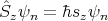
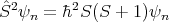
number.) The spin operator is denoted by  . There are 2 quantum numbers associated
with spin angular momentum: s and sz. Sometimes sz is denoted by ms. If spin is a
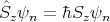
good quantum number, then the energy eigenstate ψn is also an eigenstate of Ŝ2 and
Ŝz:
. There are 2 quantum numbers associated
with spin angular momentum: s and sz. Sometimes sz is denoted by ms. If spin is a
good quantum number, then the energy eigenstate ψn is also an eigenstate of Ŝ2 and
Ŝz:
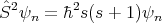 | (12) |
and
 | (13) |
(In terms of commutators, [Ĥ,Ŝ2] = 0, [Ĥ, ] = 0, and [Ŝ2,
 ] = 0.) It turns out that s
z has a
range of values:
] = 0.) It turns out that s
z has a
range of values:
 | (14) |
There are 2s + 1 values of sz. s can be either an integer or a half–integer. Particles with integer spin are called bosons and particles with half–integer spin are called fermions. An example of a fermion is an electron. An electron is a spin-1/2 particle, i.e., s = 1∕2, and it has 2 spin states: spin up (which corresponds to sz = +1∕2) and spin down (which corresponds to sz = -1∕2). Protons and neutrons are also spin–1/2 particles and are therefore fermions.
An example of a boson is a photon. A photon is a spin–1 particle, i.e, s = 1, and it has
sz = -1 or sz = +1. It turns out not to have sz = 0. This is related to the fact that there are 2
possible polarizations of the electric field  and that
  ⊥
⊥ , where
  points in the direction of
propagation of the electromagnetic wave.
points in the direction of
propagation of the electromagnetic wave.
 | (15) |
The total angular momentum also has 2 quantum numbers associated with it: S and Sz. If these are good quantum numbers, then the energy eigenstate ψn satisfies:
 | (16) |
and
 | (17) |
One can also add orbital angular momenta. The rules for angular momentum addition are the
same for all types of angular momentum. But the rules for adding angular momenta in
quantum mechanics are a little tricky. You might think that if one particle has angular
momentum s1 (be it spin or orbital or total) and another independent particle has angular
momentum s2, the total is s = s1 + s2. This is not necessarily so. Classically you don’t add two
vectors by adding their magnitudes:  1 +
1 +  2≠|s|1 + |s|2. You don’t do this in quantum
mechanics either. In quantum mechanics the rule is that if you add s1 and s2, the total s
obeys
2≠|s|1 + |s|2. You don’t do this in quantum
mechanics either. In quantum mechanics the rule is that if you add s1 and s2, the total s
obeys
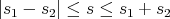 | (18) |
The z component sz still runs from -s to +s in integer steps; there are 2s + 1 values of sz. So if we add the spin angular momentum of 2 spin–1/2 particles, the total spin S of the system is S = 0 (we call this a singlet) or S = 1 (we call this a triplet). The singlet state has sz = 0 and the triplet state has 3 possible values of sz: –1, 0, +1. In this way one can make a composite particle that is a boson out of fermions. For example, 4He is a boson because if you add the spin of the proton, neutron, and 2 electrons, you always will get an integer. On the other hand 3He is a fermion.
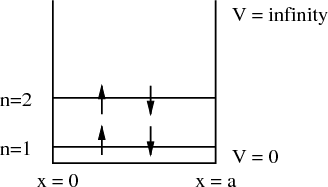
Consider the quantum mechanical problem of a box with infinitely high walls. We can label the states with quantum numbers n, spin s and the z–component of spin sz. Suppose we put 4 electrons in this box. Two electrons, one spin up and the other spin down, go into the n = 1 state. The quantum numbers of these two electrons is (n = 1, s = 1∕2, sz = 1∕2) and (n = 1, s = 1∕2, sz = -1∕2). The other two electrons go into the n = 2 state. They have quantum numbers (n = 2, s = 1∕2, sz = 1∕2) and (n = 2, s = 1∕2, sz = -1∕2).
 | (19) |
Notice that if we interchange 1 and 2, we get ψ(2, 1) = -ψ(1, 2). This is what we mean by antisymmetry. If fermions 1 and 2 were both in the same state, say ϕa, then we would get
 | (20) |
Thus antisymmetry enforces the Pauli exclusion principle. In general a wavefunction describing a collection of N fermions must be antisymmetric and satisfy
 | (21) |
Bosons are symmetric under exchange. For example, if we have 2 bosons with coordinates 1 and 2, and we put them into 2 states ϕa and ϕb, a symmetric wavefunction for them is:
 | (22) |
If we interchange 1 and 2, we get ψ(2, 1) = ψ(1, 2). This is what we mean by a symmetric wavefunction. If bosons 1 and 2 were both in the same state, say ϕa, then we would get
 | (23) |
Thus it’s ok to put more than one boson in the same single particle state. In general a wavefunction describing a collection of N bosons must be symmetric and must satisfy
 | (24) |