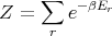
|
| (1) |
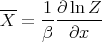
then we can derive just about anything we want to know from the partition function such as the mean internal energy, the entropy, the pressure, the Helmholtz free energy, the specific heat, etc. Let’s give some examples of how this works.
 B. Associated with this magnetic moment is the spin angular
momentum ℏ
B. Associated with this magnetic moment is the spin angular
momentum ℏ of the electron. Protons and neutrons also have angular momentum ℏ
 and magnetic moments
  . This gives rise to nuclear magnetic moments which are
involved in NMR and MRI. The magnetic moment of an atom, ion or single elementary
particle such as an electron or proton in free space is proportional to its angular
momentum:
. This gives rise to nuclear magnetic moments which are
involved in NMR and MRI. The magnetic moment of an atom, ion or single elementary
particle such as an electron or proton in free space is proportional to its angular
momentum:
 | (2) |
where the proportionality factor g is the “spectroscopic splitting” factor or just the g factor, μB
the Bohr magneton, γ the gyromagnetic ratio, and ℏ the total angular momentum. Rather
than considering the case of arbitrary
the total angular momentum. Rather
than considering the case of arbitrary  (see Reif 7.8, pages 257-262), let us begin by
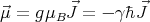
considering the simple case of spin-1/2 where J = 1∕2 and g = 2. Then the allowed quantum
energy states are
(see Reif 7.8, pages 257-262), let us begin by
considering the simple case of spin-1/2 where J = 1∕2 and g = 2. Then the allowed quantum
energy states are
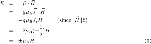
If we consider only one atom or ion, the partition function ξ of that one atom or ion becomes
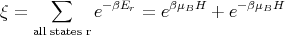 | (4) |
and
 | (5) |
The mean energy can be calculated from
 | (6) |
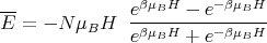 | (7) |
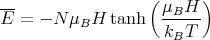 | (8) |
The total magnetic moment or magnetization can be calculated from
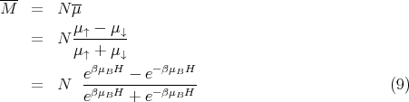
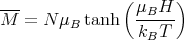 | (10) |
Alternatively we can calculate the generalized force associated with the magnetic field. Recall that
 | (11) |
and
 | (12) |
¿From Reif 11.1 we find that magnetic work is
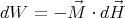 | (13) |
where  is the magnetization. Suppose
  is pointing along the ẑ axis. We can identify H with
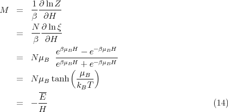
the external parameter x, and M, the z–component of
is pointing along the ẑ axis. We can identify H with
the external parameter x, and M, the z–component of  , with the generalized force. Then the
generalized force is
, with the generalized force. Then the
generalized force is
 | (15) |
We can examine M in the limit of high and low temperature.
 | (16) |
Physically at low temperatures all the magnetic moments are aligned with the magnetic field.
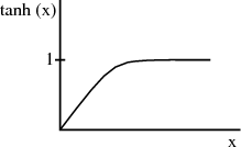
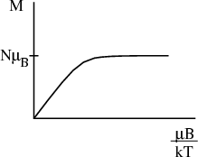
At high temperatures, μBH∕kBT → 0 and T →∞. Since tanh(x) → x as x → 0, we obtain
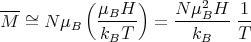 | (17) |
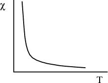
We expect the magnetization to be proportional to the magnetic field H. This is what characterizes a paramagnet. How easy or hard it is to magnetize the system is reflected in the magnetic susceptibility χ:
 | (18) |
¿From eq. (17) we can read off the susceptibility:
 | (19) |
The fact that χ varies as 1∕T is know as the Curie law. χ is called the Curie susceptibility because it goes as 1∕T.
We can also calculate the Helmholtz free energy using eqns. (5) and (4):
 | (20) |
where
 | (21) |
So
 | (22) |
We can also calculate the heat capacity. Recall from lecture 9 that
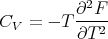 | (23) |
Taking two derivatives of (22) yields
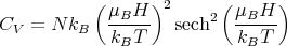 | (24) |
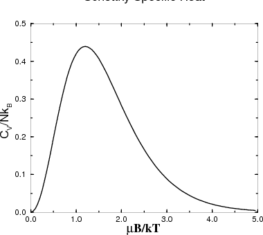
The specific heat per spin is
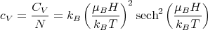 | (25) |
This is called the Schottky specific heat. It is the specific heat characteristic of two state systems. A two state system has only 2 states available to it. For example a spin–1/2 object has spin–up and spin–down states. Another example is an object that can only access the lowest states in a double well potential. In considering such discrete states, we are thinking quantum mechanically.
 | (26) |
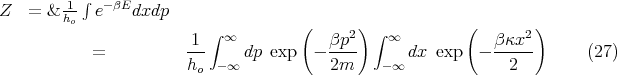
Assume the harmonic oscillator is in contact with a thermal reservoir at temperature T. The partition function is
Recall from Reif Appendix A4 that
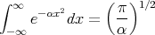 | (28) |
Using this (27) becomes
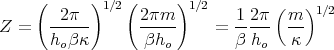 | (29) |
Or
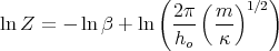 | (30) |
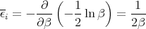
and
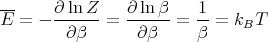 | (31) |
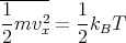
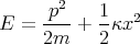
This makes sense; we expect the mean energy to be of order kBT. It turns out that E - kBT has equal contributions from the kinetic energy and from the potential energy. Each contributes kBT∕2. One can show this explicitly. The mean kinetic energy is
 Classical Equipartition Theorem Let
the energy of a system with f degrees of freedom be E = E(q1...qf,p1...pf) and
assume
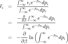
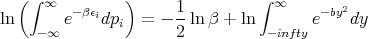
If we replaced pi by qi, the theorem is still true. We just want ϵi to be a quadratic function of one component of q or p. Assume that the system is in equilibrium at temperature T. Then 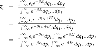
where y ≡ β1∕2p i. Thus
Notice that the integral does not involve β. So when we take the derivative in (36), only the first term is involved.
or
This is the classical equipartition theorem. It says that each additive quadratic term in the energy (i.e., each degree of freedom) contributes kBT∕2 to the mean energy of the system. Note that this theorem is true only in classical statistical mechanics as opposed to quantum mechanics. In quantum mechanics the energy of a system is discretized into energy levels. At low energies the levels are rather far apart. As the energy increases, the energy levels become more closely spaced. The equipartition theorem holds when mean energy is such that the levels near it have an energy level spacing ΔE ≪ kBT. Mean kinetic energy of a gas molecule
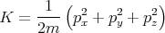
Let’s consider the simple example of a molecule in a gas (not necessarily an ideal gas) at
temperature T. Its kinetic energy is given by
The kinetic energy of the other molecules do not involve the momentum
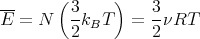
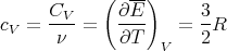
For an ideal monatomic gas the energy is solely kinetic energy, so
where N is the number of gas particles, R = NakB is the gas constant, and ν is the number of moles. The molar specific heat at constant volume is
Brownian Motion
Brownian motion was discovered by Brown, a botanist, in the 1800’s and was explained by
Einstein in 1905. If you put a small macroscopic particle in a liquid and watch it in a
microscope, it jiggles around because the molecules in the liquid keep bumping into it. This is
called Brownian motion. The molecules in the liquid are moving around because of thermal
fluctuations. To see this, let the small macroscopic particle have a mass m and be
immersed in a liquid at temperature T. Consider the x-component of the velocity
vx.
Even though the mean value of the velocity vanishes, this does not mean that vx = 0. There are velocity fluctuations so that vx2≠0. ¿From the equipartition theorem we have
or
The factor of 1∕m means that the fluctuations are negligible for large m like a golf ball. But when m is small (e.g., when the particle is micron sized), then the velocity fluctuations become appreciable and can be observed under a microscope. Notice that the size of the fluctuations are proportional to temperature. The higher the temperature, the larger the fluctuations. This is what we expect of thermal fluctuations. |


 of this particular
molecule. The potential energy of interaction between the gas molecules also is independent of
of this particular
molecule. The potential energy of interaction between the gas molecules also is independent of
 . So the equipartition theorem tells us that