Next: About this document ...
LECTURE 9
Statistical Mechanics
Basic Methods
We have talked about ensembles being large collections of copies or
clones of a system with some features being identical among all the
copies. There are three different types of ensembles in statistical mechanics.
- If the system under consideration is isolated, i.e., not interacting
with any other system, then the ensemble is called the microcanonical
ensemble. In this case the energy of the system is a constant.
- If the system under consideration is in thermal equilibrium
with a heat reservoir at temperature
 , then the ensemble is called
a canonical ensemble. In this case the energy of the system is not
a constant; the temperature is constant.
, then the ensemble is called
a canonical ensemble. In this case the energy of the system is not
a constant; the temperature is constant.
- If the system under consideration is in contact with both a heat
reservoir and a particle reservoir, then the ensemble is called
a grand canonical ensemble. In this case the energy and particle number
of the system are not constant; the temperature and the chemical
potential are constant. The chemical potential is the energy required
to add a particle to the system.
The most common ensemble encountered in doing statistical mechanics is
the canonical ensemble. We will explore many examples of the canonical
ensemble. The grand canonical ensemble is used in dealing with
quantum systems. The microcanonical ensemble is not used much because
of the difficulty in identifying and evaluating the accessible
microstates, but
we will explore one simple system (the ideal gas) as an example of
the microcanonical ensemble.
Microcanonical Ensemble
Consider an isolated system described by an energy in the range between
 and
and  , and similar appropriate ranges for external
parameters
, and similar appropriate ranges for external
parameters  . To illustrate a microcanonical ensemble,
consider only the energy parameter. Let
. To illustrate a microcanonical ensemble,
consider only the energy parameter. Let  be the total energy
of the
be the total energy
of the  th microstate. Also let
  be the probability of the
system being in the th microstate. The average energy is
be the probability of the
system being in the th microstate. The average energy is
 |
(1) |
where the sum is over the accessible microstates. From the
postulates of statistical mechanics that all microstates are
equally probable, the probability of the system being in any
microstate is a constant as long as the total energy is in the range
to . Assume there are  such states, then
 |
(2) |
The average value of any property of the system is
 |
(3) |
where  is the value of the property
  when the
system is in the th microstate. The difficulty is that identifying
the correct set of microstates is exceedingly difficult. If we think of
phase space as consisting of all possible microstates of the system
with all possible energies, then the microcanonical ensemble consists
of the subset of phase space with microstates that have energy between
and . Picking out these states is difficult. For example
consider an ideal gas. Let each gas particle be a ``system''. Each system
or particle is isolated and doesn't interact with anything. The microcanonical
ensemble would consist of those particles with kinetic energy between
and , i.e., it would consist of only those particles with
a certain velocity. We could only sum over those particles, not all
the particles. Picking out these particles is a pain.
when the
system is in the th microstate. The difficulty is that identifying
the correct set of microstates is exceedingly difficult. If we think of
phase space as consisting of all possible microstates of the system
with all possible energies, then the microcanonical ensemble consists
of the subset of phase space with microstates that have energy between
and . Picking out these states is difficult. For example
consider an ideal gas. Let each gas particle be a ``system''. Each system
or particle is isolated and doesn't interact with anything. The microcanonical
ensemble would consist of those particles with kinetic energy between
and , i.e., it would consist of only those particles with
a certain velocity. We could only sum over those particles, not all
the particles. Picking out these particles is a pain.
Canonical Ensemble
The most common situation encountered in statistical mechanics is that
of a system in thermal contact with a heat reservoir at constant
temperature . In equilibrium the system is also at temperature
. The system under consideration may be a small part of a larger system,
for example, a 1 gram block of copper immersed in a container of liquid
helium at 4.2 K.
Assume that system A is in thermal contact with a heat reservoir A .
Thermal contact means that only heat can be exchanged between A and A.
The energy of system A cannot be specified since it will fluctuate
as heat is exchanged randomly between A and A (but
.
Thermal contact means that only heat can be exchanged between A and A.
The energy of system A cannot be specified since it will fluctuate
as heat is exchanged randomly between A and A (but  will be well defined). Let be the energy of a microstate of A.
Then
will be well defined). Let be the energy of a microstate of A.
Then
 |
(4) |
where  is the energy of the heat reservoir A and
  is the total energy of the combined system A and A. The probability
of A being in microstate is proportional to the
number
is the total energy of the combined system A and A. The probability
of A being in microstate is proportional to the
number
 of microstates of the reservoir:
 |
(5) |
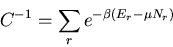
where  is a constant determined by the normalization condition:
 |
(6) |
Now assume  (i.e., assume that A is a heat
reservoir) and expand about
(i.e., assume that A is a heat
reservoir) and expand about
 :
:
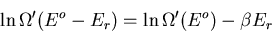
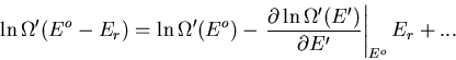 |
(7) |
But
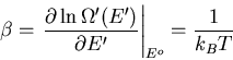 |
(8) |
where is the temperature of the reservoir. Thus
 |
(9) |
or
 |
(10) |
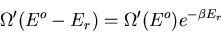
Thus
 |
(11) |
where
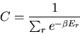 |
(12) |
Finally
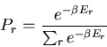 |
(13) |
This probability distribution is sometimes called the Boltzmann
distribution. It tells us the probability that a microstate with
energy will be occupied. Notice that if  , then
there is a good chance that the state will be occupied. But if
is large compared to the temperature, then the chance that the th state
is occupied is exponentially small.
, then
there is a good chance that the state will be occupied. But if
is large compared to the temperature, then the chance that the th state
is occupied is exponentially small.
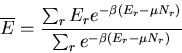
The average value of any parameter is given by
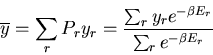 |
(14) |
where is the value of the parameter in the th state.
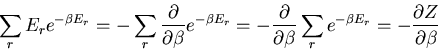
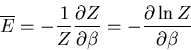
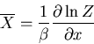
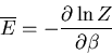
For example, the mean energy is
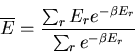 |
(15) |
The denominator arises quite frequently. So let
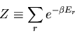 |
(16) |
 is called the partition function. It acts like a generating
function. For example,
is called the partition function. It acts like a generating
function. For example,
 |
(17) |
or
 |
(18) |
The partition function is quite useful and we can use it
to generate all sorts of information about the statistical mechanics
of the system.
The advantage of the canonical ensemble should now be apparent. The sum
is over all the microstates of the system. We don't have the
difficulty of finding only those microstates whose energy lies within
some specified range.
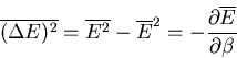
Let us also calculate the dispersion
 of the
energy:
of the
energy:
 |
(19) |
We have already computed . We need now to compute
 :
:
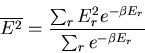 |
(20) |
But
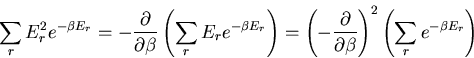 |
(21) |
And from the definition of the partition function
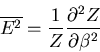 |
(22) |
This can be rewritten as
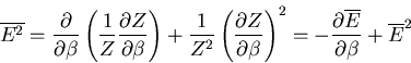 |
(23) |
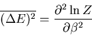
Finally we obtain
 |
(24) |
or
 |
(25) |
We can also use to generate the mean generalized force  .
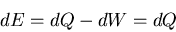
Suppose now that we change some macroscopic parameter
.
Suppose now that we change some macroscopic parameter  . Then the energy
changes by the amount
. Then the energy
changes by the amount
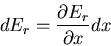 |
(26) |
and the macroscopic work done by the system is
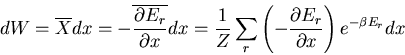 |
(27) |
Now note that in the numerator
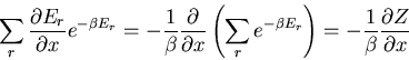 |
(28) |
Substituting in (27), we obtain
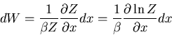 |
(29) |
Recall that
 |
(30) |
where is the generalized force associated with the parameter
:
 |
(31) |
Thus, comparing (29) and (30) leads to
 |
(32) |
If is the volume, then is the pressure  :
:
 |
(33) |
Now let's derive a relation between  and . Note that is a function
of both
and . Note that is a function
of both  and . Thus
or
 |
(35) |
But since
 |
(36) |
we obtain
 |
(37) |
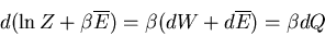
or
 |
(38) |
or
 |
(39) |
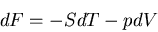
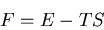
Recall that in thermodynamics
 where
where  is the
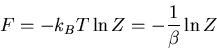
Helmholtz free energy. Hence
is the
Helmholtz free energy. Hence
 |
(40) |
or
 |
(41) |
This equation forms the bridge between the canonical ensemble of statistical
mechanics and thermodynamics. We can use it to relate the microscopics of
the system to the macroscopic parameters that we deal with in thermodynamics.
Notice that since
 |
(42) |
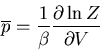
we can write the mean pressure as
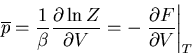 |
(43) |
We obtained this previously using
 |
(44) |
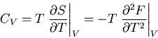
We will relate one final quantity to the partition function: the specific
heat at constant volume. Recall that
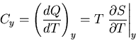 |
(45) |
Let  , then at constant volume
 |
(46) |
since 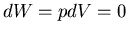 . Thus
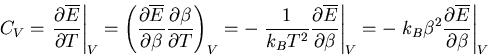 |
(47) |
But
 |
(48) |
Therefore
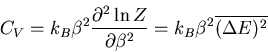 |
(49) |
Notice that the specific heat is related to the fluctuations in the
internal energy or, equivalently, to the width of the distribution of .
In a numerical simulation, one way to calculate the specific heat is
to calculate
.
We now see that the partition function contains the information about the
system. Most quantities of interest are obtained from the appropriate
derivatives of . The real task in statistical mechanics is to calculate
the partition function. Once that is done, all that remains is differentiation.
We can also relate the specific heat to the Helmholtz free energy:
 |
(50) |
Recall that
|
(51) |
implies that
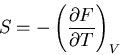 |
(52) |
We got this when we derived  using a Legendre transformation.
We can obtain the specific heat
using a Legendre transformation.
We can obtain the specific heat  using
using
 |
(53) |
This is equivalent to eq. (49).
Grand Canonical Ensemble
Suppose that the system under consideration is in contact with both a
particle and energy reservoir. In this case both energy and particle
number can be exchanged with the reservoir. In this situation neither
the total energy nor the particle number of the system is constant. Two
examples of such systems are a liter of air within a larger volume of
air, and a 1 cm sample of copper within a larger block of copper.
For mathematical reasons quantum mechanical systems are most easily
treated when in contact with both a heat and particle number reservoir.
sample of copper within a larger block of copper.
For mathematical reasons quantum mechanical systems are most easily
treated when in contact with both a heat and particle number reservoir.
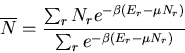
Assume that system A can exchange both energy and particles with system
A. Assume
Let
 be the number of microstates
accessible to the reservoir A when it has energy and contains
be the number of microstates
accessible to the reservoir A when it has energy and contains
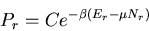
 particles. The probability of finding A in the microstate
is
particles. The probability of finding A in the microstate
is
 |
(55) |
where is a constant. Since both and
 ,
,
 |
(56) |
Let
 |
(57) |
and
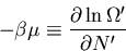 |
(58) |
where  is called the chemical potential. Note that both
and are properties of the reservoir and not the system A.
If we use the chain rule, then
is called the chemical potential. Note that both
and are properties of the reservoir and not the system A.
If we use the chain rule, then
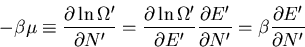 |
(59) |
This implies that
 |
(60) |
This is consistent with the statement that the chemical potential
is the energy required to add a particle or the difference in energy
between having and  particles.
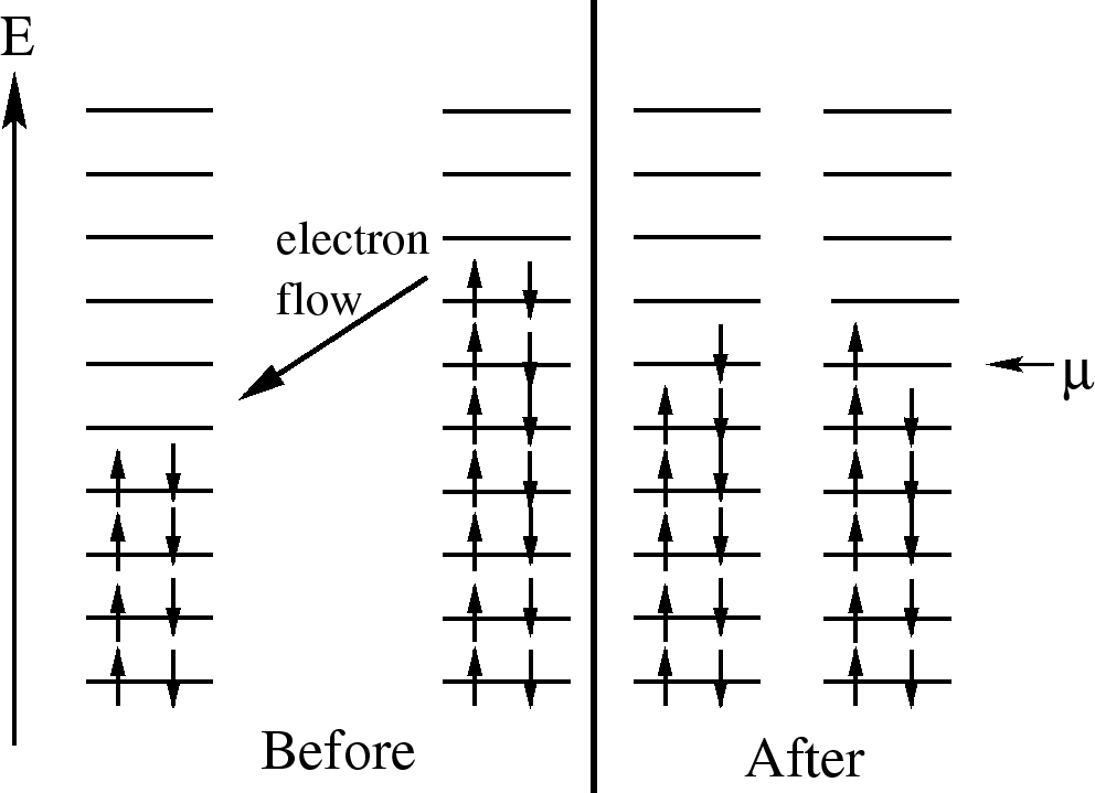
One way to think about chemical
potential is in terms of energy levels of 2 pieces of metal.
If the two pieces have different numbers of electrons, when they
are put into contact, electrons will flow from one to the other because
electrons in a higher energy level in one metal can lower their energy
by going to a lower level in the other metal. This flow continues until
the electrons are filled up to the same level. This ``level'' is the
chemical potential.
particles.
One way to think about chemical
potential is in terms of energy levels of 2 pieces of metal.
If the two pieces have different numbers of electrons, when they
are put into contact, electrons will flow from one to the other because
electrons in a higher energy level in one metal can lower their energy
by going to a lower level in the other metal. This flow continues until
the electrons are filled up to the same level. This ``level'' is the
chemical potential.
=3.0 true in
Back to (56):
 |
(61) |
and
 |
(62) |
where
 |
(63) |
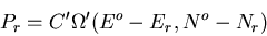
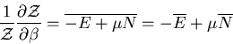
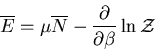
It then follows that
 |
(64) |
and
 |
(65) |
Let
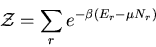 |
(66) |
Then
 |
(67) |
Also
 |
(68) |
or
 |
(69) |
or
 |
(70) |
The function  is called the grand partition function. It is this
function which is of primary importance in the grand canonical ensemble.
We will return to a consideration of the grand canonical partition function
when we begin our study of quantum statistical mechanics.
is called the grand partition function. It is this
function which is of primary importance in the grand canonical ensemble.
We will return to a consideration of the grand canonical partition function
when we begin our study of quantum statistical mechanics.
Before we begin a discussion of the applications of
these basic concepts, two useful remarks need to be made. The first is
the definition of the partition function within classical mechanics. In
clasical mechanics, the sum over microstates is replaced by an integral
over phase space. That is
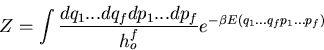 |
(71) |
A second remark concerns the partition function of two independent systems.
Let A and B be two independent systems both in contact with the same
reservoir A. Let us label the microstates of system A by and the
microstates of system B by  . We will assume that the total energy
 of system A in microstate and system B in microstate is
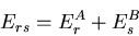 |
(72) |
The partition function of the combined system A plus B is
Thus the partition function of two independent systems is just the
product of the two independent partition functions. The only assumption
has been that the energy of the total system can be expressed as the sum
of the energies of the two individual independent systems. Notice that
this means we can add free energies:
 |
(74) |
The generalization to more than two systems is obvious. Assume we have  identical but independent systems. If
  is the partition function of
one system, then the total partition function of systems is
is the partition function of
one system, then the total partition function of systems is
 |
(75) |
We will find that quantum mechanics will lead to a correction to this
equation under certain conditions.
Next: About this document ...
Clare Yu
2007-05-15